Home
/
Blog
/
Learn the Best Google Sheets Functions!

Learn the Best Google Sheets Functions!

Google is the best thing that could have possibly happened to mankind in so many centuries. Not only Search engines, but Google also provides various amazing things like Blogger, website and wiki creation (Sites), Google Docs, YouTube, and much more.

We’ve already explored Microsoft Excel functions and features in the previous article.

Google Sheets is one such amazing product. It has been the best alternative to Microsoft Office because of its easy-to-use interface, the ability to collaborate with people, and various other functions. This article is about amazing Google Sheets functions you probably didn’t know. These google sheets features will definitely blow you by surprise. The following are some cool features of google sheets.

1. GOOGLEFINANCE

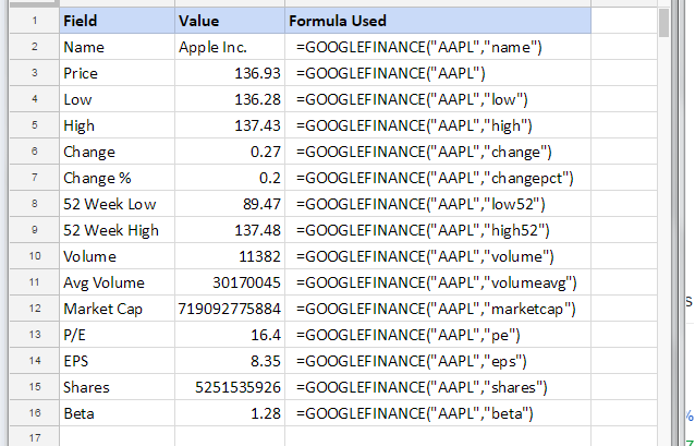
This feature fetches current and historical financial data from Google Finance to a Google Sheet. In short, this feature allows users to fetch real-time securities data from the Google Finance web application. This is one of the coolest functions of google sheets. Following is the syntax of this feature.

Syntax: GOOGLEFINANCE(ticker, [attribute], [start_date], [end_date|num_days], [interval])

where –>

Ticker: The ticker symbol for the security to consider.
Attribute: (Optional – “price” by default ) – The attribute to fetch about ticker from Google Finance.
Start_date: (Optional) – The start date when fetching historical data.
End_date num_days: (Optional) – The end date when fetching historical data, or the number of days from start_date for which to return data.
Interval: (Optional)- The frequency of returned data; either “DAILY” or “WEEKLY”.

The following image is showing us the use of GOOGLEFINANCE.

In the above example, we have used “AAPL” (Apple Inc.) for the ticker. Now after that, navigate to the Google Finance website, and enter “AAPL” in the search box, and hit the Enter key. It will display all the current stock indicators of Apple Inc. Now open the Google Spreadsheet and enter the GOOGLEFINANCE formula as shown in the above figure. It fetches all the data in the value column from the google finance website.

2. Script Functions

Google Sheets script function is the most useful weapon of the Google Spreadsheet. Google Sheets usually provide numerous built-in Microsoft Excel functions like AVERAGE, SUM, and VLOOKUP. If you feel these functions are not enough then you can use Google Apps Script to write custom functions.

For example, if you want to convert meters to miles or retrieve live data from the Internet then you can use custom functions in Google Sheets just like a built-in function. These functions are created using standard JavaScript.

Here’s a simple custom function, named MYSCRIPT, which multiplies an input value by 3:

function MYSCRIPT(input) {

return input * 3;

}

Follow these steps to create a custom function:

Open a spreadsheet in Google Sheets.
Select the menu item Tools > Script editor >Click Blank Project.
Delete any code in the script editor. For the MYSCRIPT function above, simply copy and paste the code into the script editor.
Select the menu item File > Save. Give the script project a name and click OK.
Now you can use the custom function.

After this:

Click the cell where you want to use the function.
Type an equals sign (=) followed by the function name and an input value — for example, =MYSCRIPT(A1) — and press Enter.
The cell will return the result.

3. Date functions

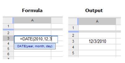
This function converts a year, month, and day into a date. In this function, every parameter should be a numeric value representing the year, month, day.

Syntax:

DATE(year, month, day)

year – The year component of the date.
month – The month component of the date.
day – The day component of the date.

If you enter a string then the #VALUE! the error will be returned. The following image is showing us the use of the date function in Google sheets.

4. Multiple Google Forms in One Spreadsheet

This is one of the coolest features of Google spreadsheets. Not many people know that they can combine multiple Google forms into one spreadsheet. Now to achieve this you can use the =importrange() function.

This feature will allow you to mirror the data from one spreadsheet to another. This is like the mirroring of a spreadsheet. In short, changes made in one spreadsheet will also be visible in another spreadsheet.

Go to tools and click on create a form.
Now you need a master spreadsheet that will display the data from multiple Google Forms. For this, create a new blank spreadsheet or the one already created by Google forms.
Now, In the master spreadsheet create a sheet for each Forms data you want to import. You can create a new sheet by clicking on the plus icon in the bottom left of the sheet.
Now, copy the URL of the spreadsheet that contains form data.
Now in the master spreadsheet select the tab where you want to display the forms data. Suppose you want to display data in A1, then in cell A1 type the formula =importrange(“URL”,“ Range”). Now replace the URL with the URL from the other spreadsheet, or the copied URL.

Example:

On the master spreadsheet, select the tab and cell you want to import data. The formula is as follows:

=importrange(“https://docs.google.com/spreadsheets/d/1KRKR-pxt1HTEEXeLwPTgGP4gt69nggcCV6TIwUJfC34/edit#gid=540243635″,”Form Responses 1!A1:D”)

5. ByteScout Lines Sorter & Cleaner

Add-ons are the most popular approach adopted by end-users in order to enhance the productivity of Google Sheets. There are a few amazing add-ons that help users to achieve their desired results efficiently and precisely. One of them is the ByteScout Lines Sorter & Cleaner.

This add-on helps users to sort text lines and lists!. With the help of this one can sort A to Z, Z to A, also sort by numbers, by names. It also enables users to clean text like trim, remove duplicates, empty lines, and much more.

Follow these steps to use this add-on in your Google Sheet.

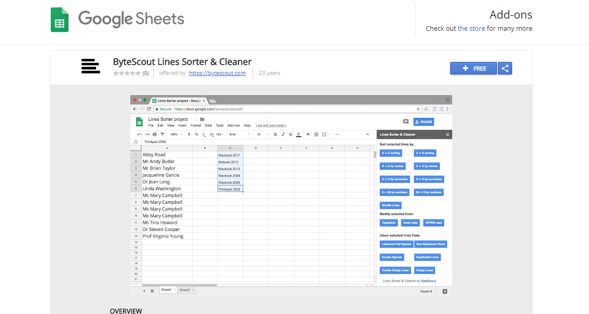
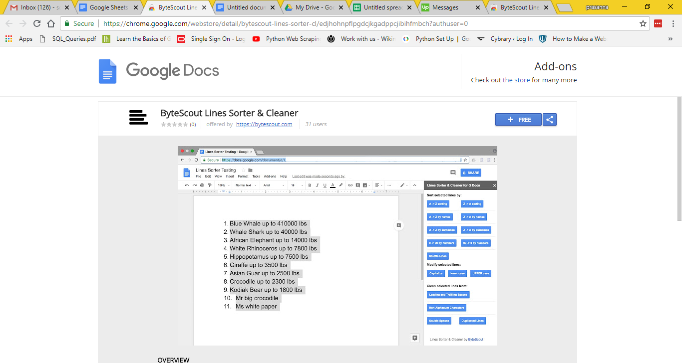
To add this to your Google Spreadsheet, go to Google Chrome Store.
Now, it will show you the following page.

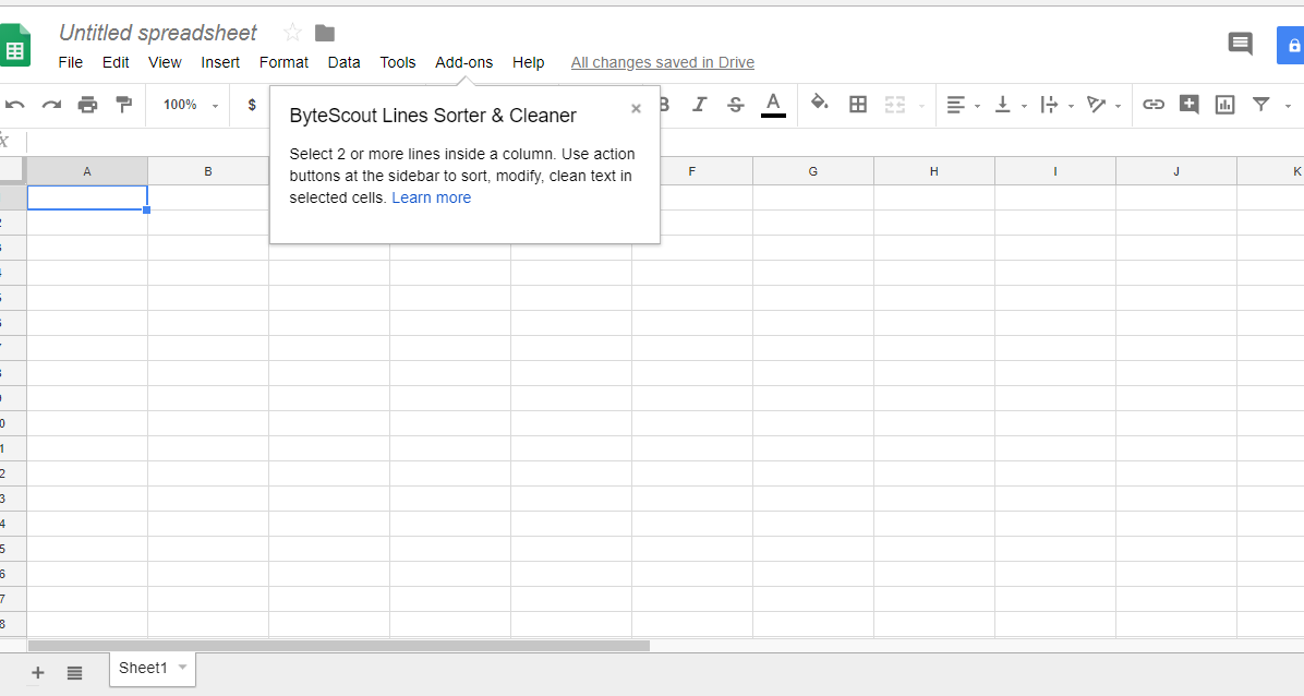
Now click on that “FREE” button to insert this add-on in your Google Sheet. When you click on this it will ask you for the necessary permission and once granted it will be added to your sheet as shown in the following figure:

Now let’s add some data to the spreadsheet and use this amazing tool. In the following Google Sheet, we have added some names in the column Name. Now, to use this Select the column/cell you want to apply this add-on and then click on Add-Ons>ByteScout Lines Sorter & Cleaner>Start

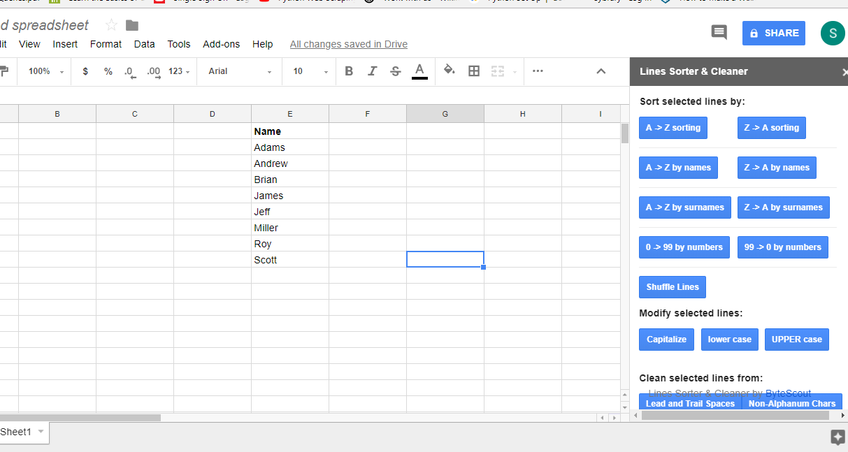
Now the following figure is showing us various functions available in Sorter & Cleaner add-on. On the right side, it is showing various functions available in this tool.

Now the following figure is displaying the use of the A>Z sorting function. This function will sort the values in the column alphabetically.

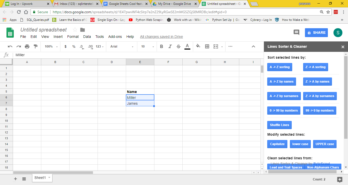
The following figure is showing us the use of the Shuffle line feature of this tool. It will cause (two or more things) to exchange places. In short, it is the transpose of cell data. The following figure is showing us the use of this feature.

The Shuffle line function above has transposed the values in E6 and E7 cells. As shown in the above figure there are three other functions available in this tool. These are Capitalize, lowercase, and uppercase. If you click the capitalize button it will change the case of the text to proper case or you can say sentence case, if you click lowercase then it will convert it into lowercase and if you click on the uppercase button then it will convert the text in uppercase. If you closely observe you will see a few more buttons on the right side of your google sheet.

These are also very useful functions. If you want to remove duplicate values from your spreadsheet then Duplicated lines button will do it for you. Just select the rows which have duplicate values and click the Duplicated lines button. All duplicate values will be removed. Now, if you want to remove empty lines or empty rows from your google sheet then this tool is a just perfect weapon. In short, if you want to remove two empty rows from your spreadsheet then use this tool.

You can also use ByteScout Lines Sorter & Cleaner plugin in Google docs, let’s see how it works.

To add this to your Google document, go to Chrome Store.
Now, it will show you the following page.

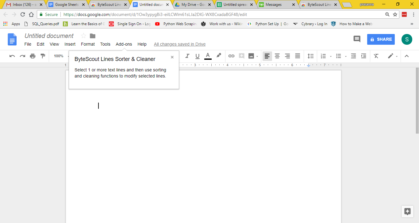
Now click on that “FREE” button to insert this add-on in your Google document. When you click on this it will ask you for the necessary permission and once granted it will be added to your document as shown in the following figure:

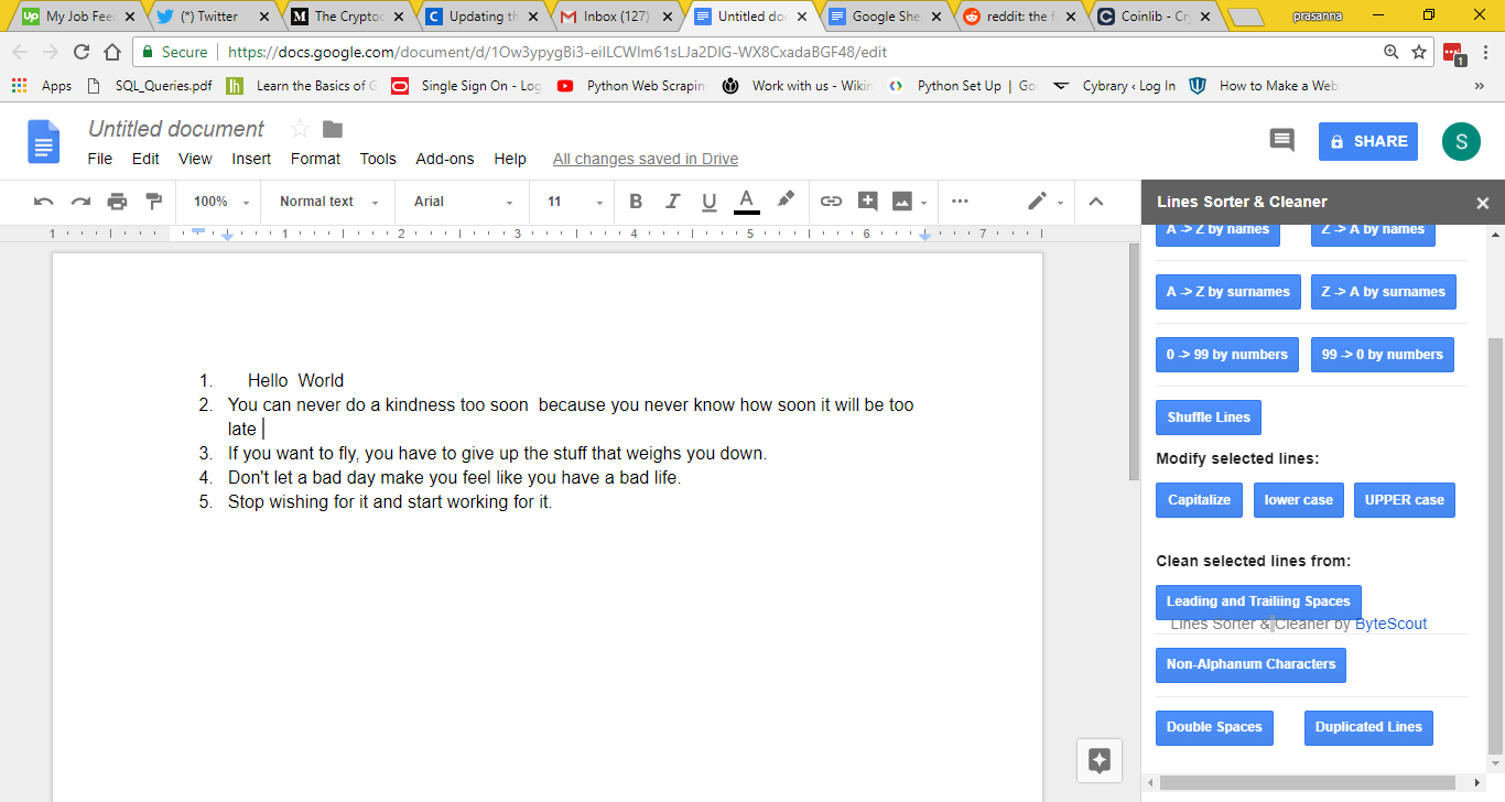
Now let’s add some data in the doc and use this amazing tool. In the following image, we have added some quotes. Now, to use this Select the quote you want to apply this add-on and then click on Add-Ons>ByteScout Lines Sorter & Cleaner>Start

The sorting function will sort as explained earlier. The capitalize, lowercase and uppercase functions will convert the case of sentences. The next function is leading and trailing space which will trim the leading and trailing spaces present in your text. The double space function will remove the spaces present while the duplicate lines function will remove all the duplicate text present in your text. If you want to arrange or sort the text of your sentence or if you have inserted a table in your Google document the sorting functions present in this tool will do that magic for you.

One of the coolest things about the Lines Sorter & Cleaner tool is that it is very easy to install and use. It is full of such functions which are always useful if you are playing with huge text or numeric data in both google spreadsheets and google documents. ByteScout Lines Sorter & Cleaner tool is a shiny new set of tools for Documents and Spreadsheets.

6. Google Sheets Query function

Google sheets query function is the most powerful function in the Google Spreadsheet. It allows you to write SQL (Structured Query Language) code to manipulate or retrieve data from the database or you can say the Spreadsheet. It is arguably the finest function in Google Sheets. Let’s take a look at it.

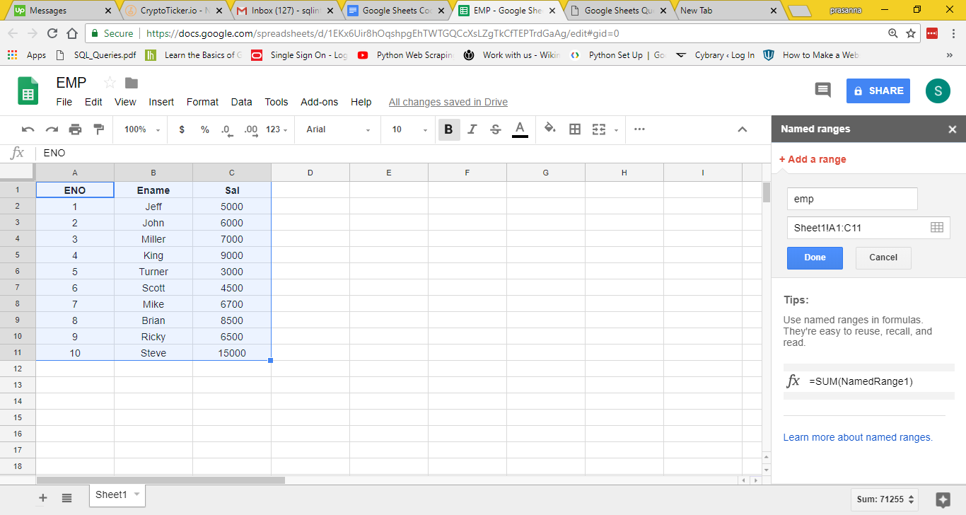
Open Google Spreadsheet and enter some data in it. In the below figure, I have created an EMP table that has three columns. This table is showing us employee numbers, employee name, and their salary. Also, select the complete table.
Now Go to the menu and then Data and then click the Named ranges option. A new window will be visible on the right side of the spreadsheet as shown below:

Now, In the input box, enter the name of our table “emp”, as shown in the image below. This names our table of data.

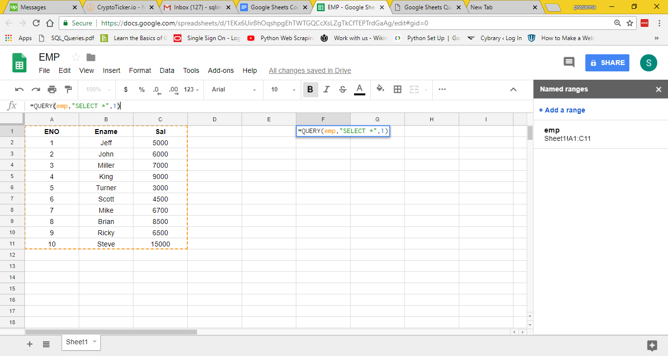
Now, in Google Sheets, we can use the Google Sheets QUERY function to write SQL code. So, now enter SQL code inside a QUERY function in cell F1. In our table, we have three columns but if you want to see the complete data then we have to write QUERY function like Select * from <table name> in google spreadsheet as shown below.

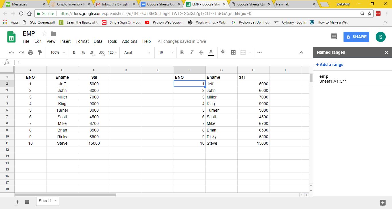
After inserting the formula in the F1 cell, press enter. It will display the following result.

The above figure is showing us various dates in the date column. The value in cell D2 is 7/22/2018. It displayed because we entered the formula =TODAY() function in the D2 cell. In short, the TODAY function will always display the current system date. Now, enter =TODAY()+30 this will display the date 8/21/2018. We have simply added 30 days in date function. Now if you add 100 days in the date function it will display 10/30/2018 as shown in the above figure.

7. IMPORTHTML

This function imports data from a table or list within an HTML page.

Syntax:

IMPORTHTML(url, query, index)

where

Url: The URL of the page to include in your spreadsheet including protocol (e.g. http://). The value of the URL should be enclosed in quotation marks.

Query: If you want to insert “list” or “table” from the website in your spreadsheet then you have to clearly mention it as either “list” or table here.

Index – The index which will start at 1. It identifies which table or list as mentioned in the HTML source should be returned. The index is an indicator or measure of something.

Example:

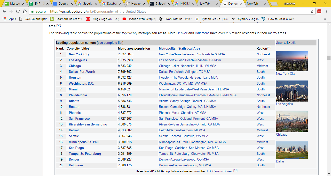
Now, if you want to import some data from a website in a database then this function is useful. Now, the following table is showing us the populations of the top twenty metropolitan areas in the USA. It is available on the Wikipedia page.

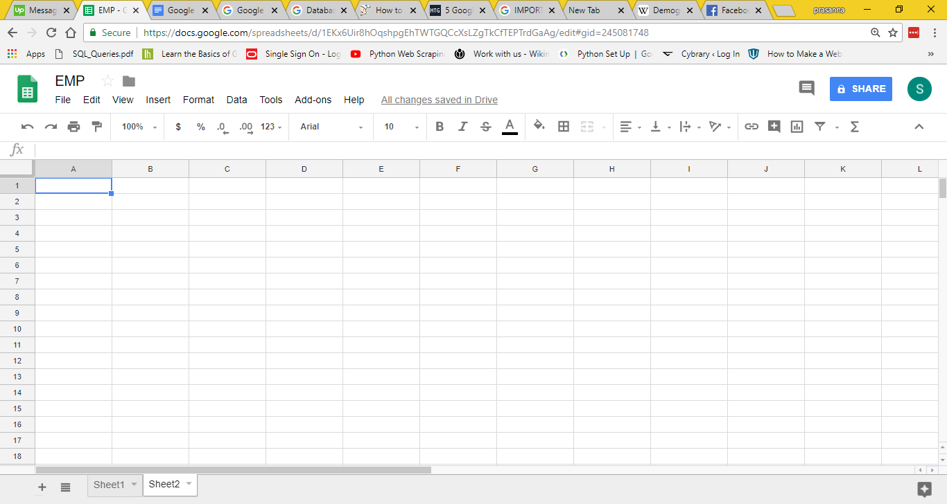
We want to import the data shown above in our google spreadsheet. To import this table into a spreadsheet open a blank spreadsheet as shown in the below figure.

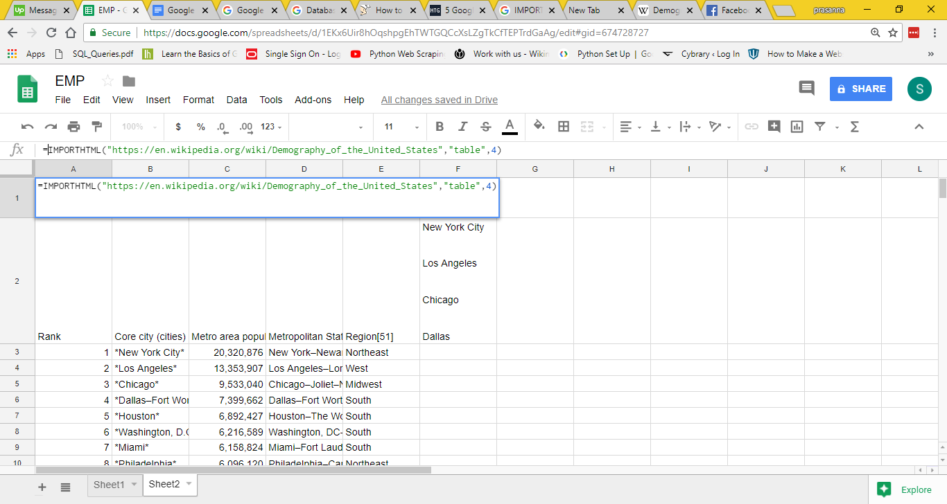
Now insert =IMPORTHTML(“https://en.wikipedia.org/wiki/Demography_of_the_United_States”,”table”,4) in cell A1. This function will import data from the Wikipedia page. The index is 4. This is because the table shown above is the fourth table present on the Wikipedia page and we want to import this table into our spreadsheet. The following image is showing how to insert this function in a Google Spreadsheet and to get the result by pressing Enter.

8. GOOGLETRANSLATE

Many people have used google translate to translate website content but many people don’t know that this function can also be used in Google Spreadsheet. If you want to translate value from a particular cell into a specific language then Googletranslate function is amazing.

Syntax:

GOOGLETRANSLATE(text, [source_language], [target_language])

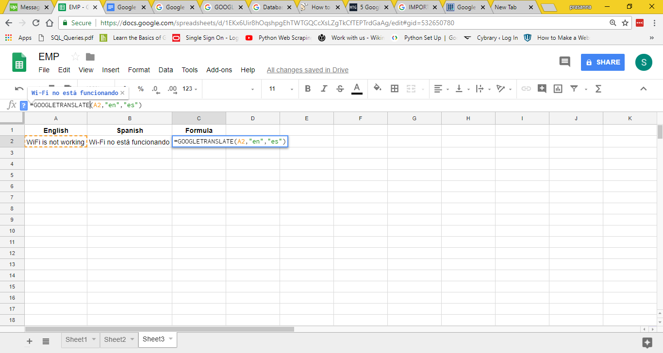
For example: the following figure is showing some text entered in cell A1. If you want to convert this text is French language or any other language then this function can be used.

The above figure is showing us the desired result. It has converted the text into English and Spanish. For this, we have entered the below formula in cell B2.

=GOOGLETRANSLATE(A2,”en”,”es”). Google Translate doesn’t translate all of the 6,000+ languages but it does translate the most commonly used languages. For more information, you check google’s documentation.

There are many more fancy tricks in Google Sheets. Stay tuned!