Our ByteScout SDK products are sunsetting as we focus on expanding new solutions.
Learn More
Important Update
ByteScout SDK Sunsetting Notice
Our ByteScout SDK products are sunsetting as we focus on our new & improved solutions.Thank you for being part of our journey, and we look forward to supporting you in this next chapter!
Learn TOP-40 Excel Advanced Features and Functions in 2023
Learn TOP-40 Excel Advanced Features and Functions in 2023
Microsoft Office Excel is one of the most important tools to perform the calculation, analysis, and visualization of data and information. It helps people to organize and process data by the use of columns and rows with formulas and some cool features of MS Excel. In MS-Excel 2010, row numbers range from 1 to 1048576. There are a total of 1048576 rows, and columns range from A to XFD and there are a total of 16384 columns. Now, let’s take a closer look at some of the best Microsoft Excel features or functions you can use to become more efficient.
This function helps to search for a value in a table. It returns a corresponding value. In other words, it searches for the given value and returns a matching value from another column. To know more about it, let’s look at the following syntax and its example.
In the above syntax, lookup_value is the value to search for. It can be text, date, or number. Table_array is two or more data columns. Col_index_num is the column number in table_array from which the value in the comparable row should be returned.
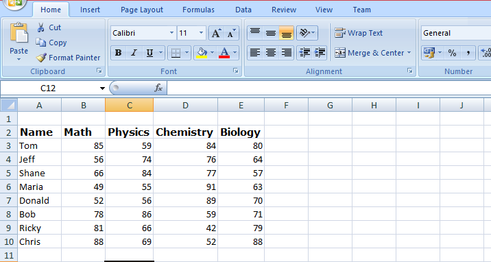
Example:In the below example we have student names and marks in different subjects in columns B to E.
From the above data, we need to know how much Ricky scored in Math.
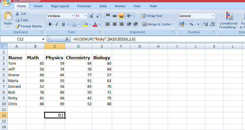
Here is the VLOOKUP formula that will return Ricky’s Math score:
=VLOOKUP("Ricky",$A$3:$E$10,2,0)
First, it looks for the value of Ricky in the Name column. It goes from top to bottom and finds the value in cell A9. After that, as soon as it finds the value of the Math score, it goes to the right in the second column (Math) and fetches the value in it. The following picture shows us Ricky’s marks.
Check out this little demo to see how you can use the VLOOKUP formula:
2. Pie Chart
The pie chart is one of the best MS Excel features. It is used to visualize the contribution of each value to a complete pie diagram. It always uses one data series.
Follow the below steps to create a pie chart:
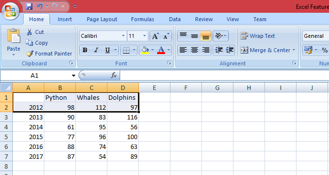
Select the range A1: D2.
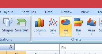
Now On the Insert tab, in the Charts group, click the Pie symbol and then click Pie.
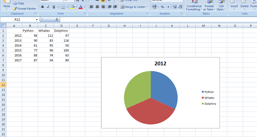
After clicking, the following image will show the result.
The above figure shows us the pie chart for the year 2012. It is showing us the Python slice, Whales slice, and Dolphins’ slice. In short, the contribution of each slice.
Please find a comprehensive demo where you can see how the pie chart can be used:
3. Mixed or Combination Type Charts
A mixed or combination chart is one of the top features of MS Excel. It combines and displays two or more chart types in a single chart. To create a combination chart follow the following steps:
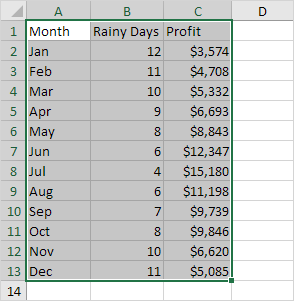
Select the range A1: C13.
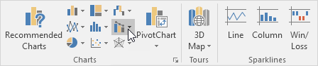
Now, On the Insert tab, in the Charts group, click the Combo symbol, and after that click on create custom combo chart.
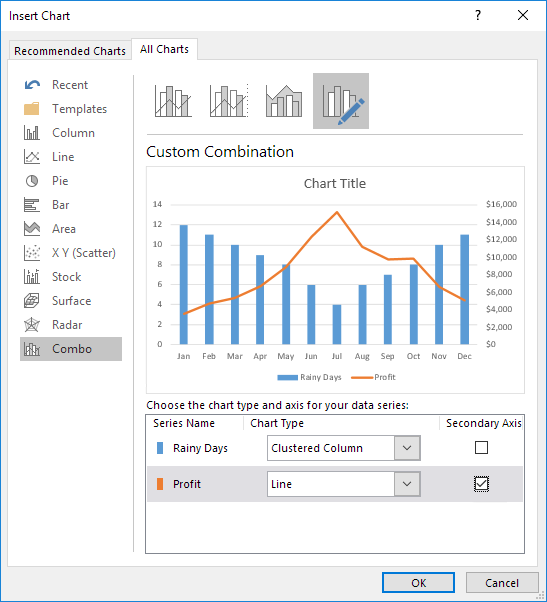
Now, the insert chart dialogue box will appear. Now, for the rainy days series, select the clustered column as the chart type. After that for the profit series, select line chart type. Now, plot the profit series on the secondary axis.
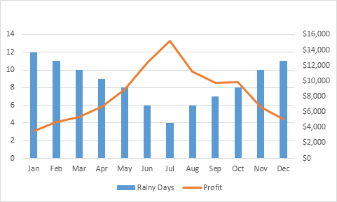
After clicking OK, it will display the following result:
A mixed or combination chart is one of the coolest Microsoft Excel advanced features and functions.
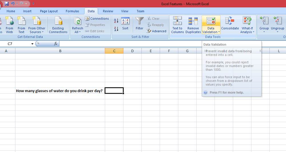
4. Data Validation
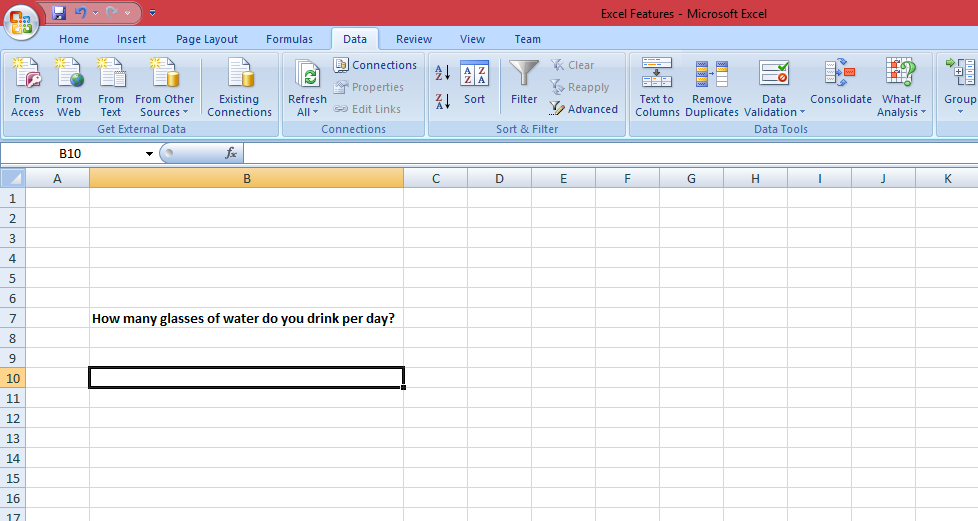
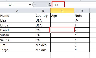
Data validation is one of the most powerful excel capabilities. It makes sure that users enter particular values into a cell. In the following example, we have restricted users to enter a whole number between 0 and 10.
Now, to create Data Validation Rule, Select cell C7 and now on the Data tab, in the Data Tools group, click Data Validation.
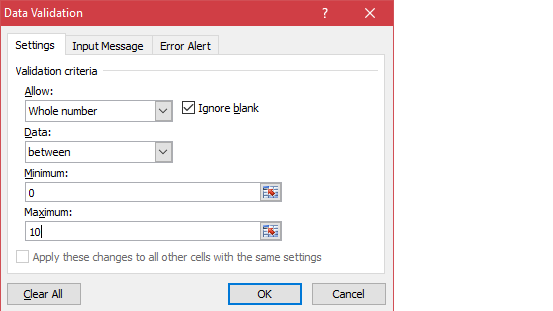
Now, On the Settings tab, in the allow list, click the Whole number, and after that in the data list, click between. Now enter the minimum and maximum values.
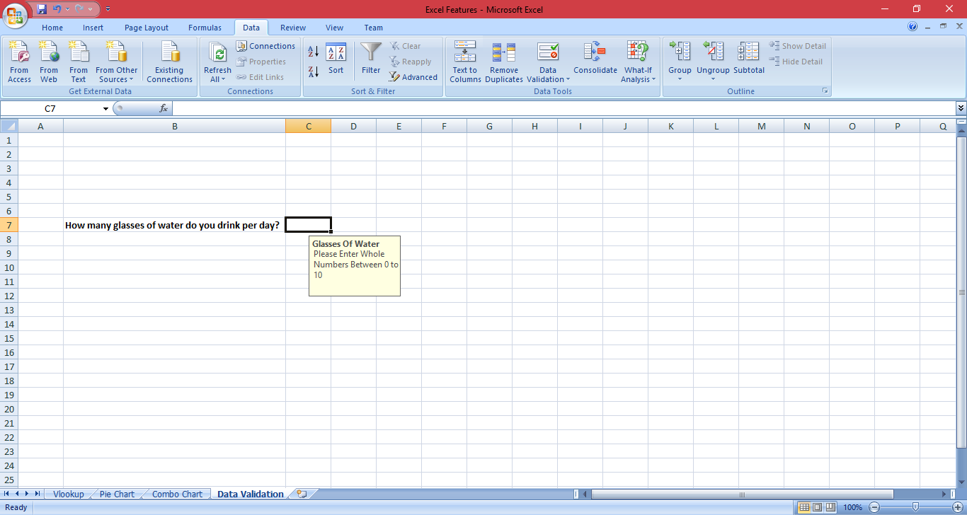
Now, after this click on Input Message and set the input message. After finishing this click on the Error Alert tab and set the error message to display if a user enters other than whole numbers or some other text. The following two figures show you the result.
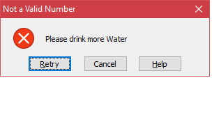
Now, try to enter a number higher than 10. The following image is showing us the result:
5. IFERROR Function
If you are in the field of data analysis then IFERROR is one of the coolest advanced Excel formulas and functions. It returns a result when a formula generates an error and a typical result when no error is found. IFERROR is a simple way to manage errors without using more complex nested IF statements.
Syntax
=IFERROR (value, value_if_error)
Example:
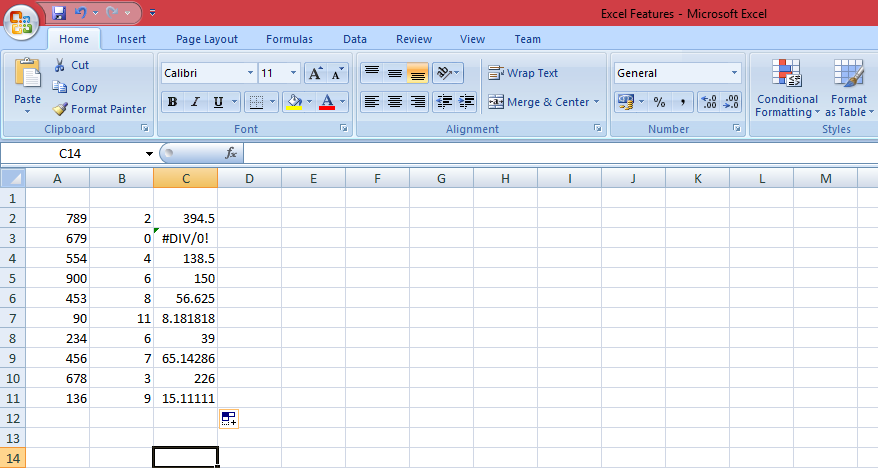
The following example will show the use of IFERROR function. This example displays the #DIV/0! error when a formula tries to divide a number by 0.
Now if we use iferror function then if a cell contains an error, an empty string (“”) is displayed.
6. Remove Duplicates
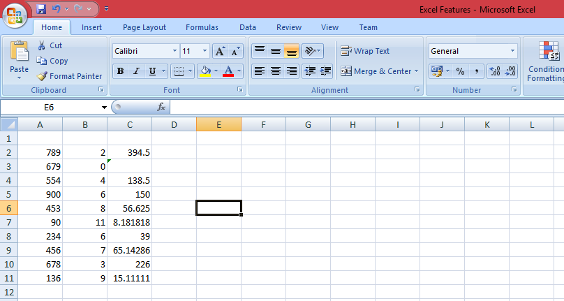
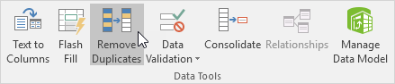
Removing duplicates is the most powerful ms excel feature for people who work as data analyst or those who play with data regularly. This example shows you how to remove duplicates in Excel. Check the following example. Click any single cell inside the data set and on the Data tab, in the Data Tools group, click Remove Duplicates.
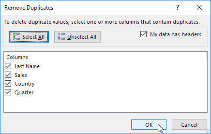
The following dialogue box will appear. Now, leave all checkboxes checked and click OK.
MS Excel will remove all identical rows (blue) except for the first same row.
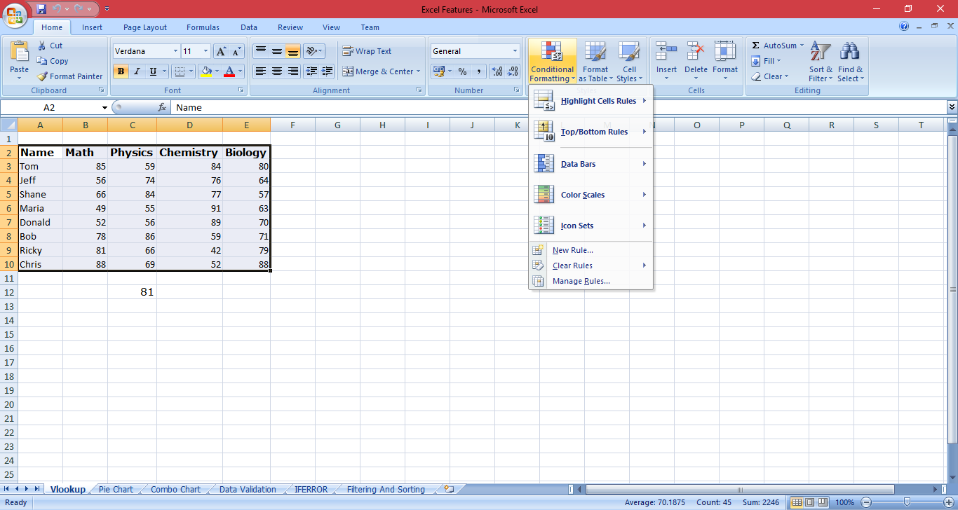
Conditional formatting allows a user to change the format of a cell depending on the content of the cell, a range of cells, or another cell or cells in the spreadsheet. It also allows users to highlight errors and find important patterns in data. Conditional formats can apply basic font and cell formattings like number format, font color, and other font properties, cell borders, and cell color. Also, there are different conditional formats that allow visualizing data by using icon sets, color scales, or data bars.
8. MINVERSE
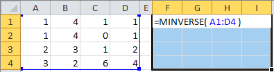
The Microsoft Excel MINVERSE function gives the inverse matrix of a given matrix. This function comes under Math/Trig Function.
Syntax: MINVERSE( array )
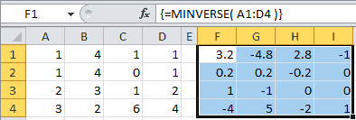
In the below example, the minverse function is entered into cell F1 of the spreadsheet. It will be like =MINVERSE( A1: D4 ). Check the following images for a result.
The result is displayed in cells from F1 to I4.
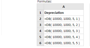
9. DB Function
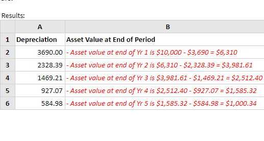
Microsoft Excel DB function is a financial function. It allows users to calculate the depreciation of an asset. In this, the fixed-declining balance method for each period of the asset’s lifetime is used.
Syntax=DB(cost, salvage, life, period, [month])
In the following spreadsheet, the DB function is finding the yearly depreciation of an asset that costs $10,000 at the start of year 1, and has a salvage value of $1,000 after 5 years.
Now after entering the above formulas in each cell the following figure is showing us the result.
10. Data Visualization
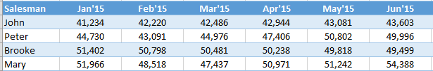
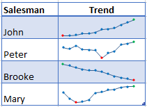
Data is the new oil and data visualization is also one of the most powerful Microsoft Excel features. Sparkline is an amazing excel feature. It is also called a visualization tool for MS Excel that enables people to perfectly visualize the overall trend of a set of values. In short, sparklines are mini-graphs situated inside cells. The following example will show you sparklines.
To create the sparklines, follow these steps Select the range that contains the data that you’ll plot. Now, Go to Insert > Sparklines > Select the type of sparkline you want (Line, Column, or Win/Loss). In the above example, we are using lines. Check the below image to see the result:
11. Complex Function
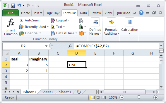
COMPLEX function converts real and imaginary coefficients into a complex number like x + yi or x + yj.
The following image is showing us the conversion. If you write =COMPLEX(A2, B2) in the D2 cell then it will convert a real and imaginary number into a complex number 3+5i as shown in the figure.
12. MKDIR
Yes, MKDIR exists in MS Excel and it is one of the most underrated excel capabilities. It comes under the File/Directory Function. MKDIR can be used as a VBA function. It can be used in macro code that is entered through the Microsoft Visual Basic Editor.
Syntax: MkDir path
Example: MkDir “c:\Sample\Excel2010”
The MKDIR command will only create the Excel2010 directory under the c:\Sample directory. It will not create the c:\Sample folder automatically.
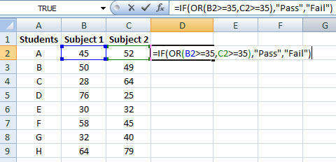
13. IF and OR function
If you want a binary result in excel then the If and Or function is useful. In short, if you want to achieve True or False or Pass or Fail as a result then If or function can be used. In this, our formula starts with an IF function, and in that, we embed the OR function. See the below image.
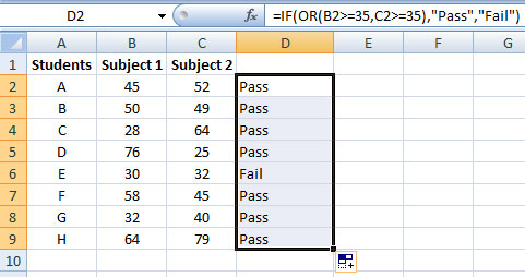
Now when you press enter and drag the fill handle, the Pass or Fail result will be displayed. Check the below image.
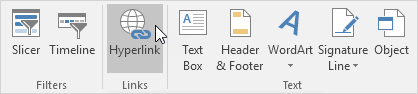
14. Hyperlink
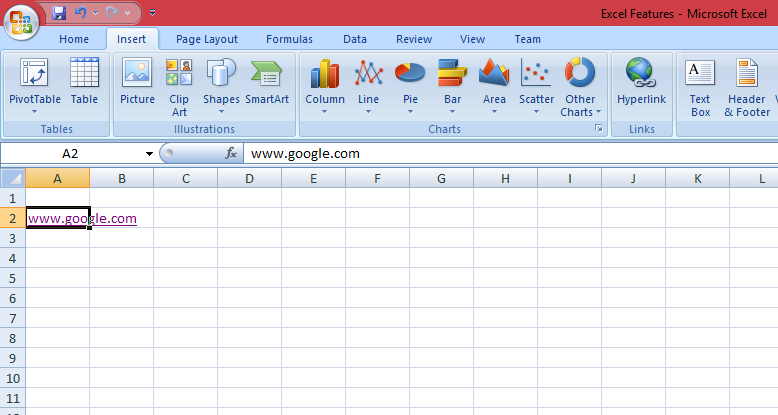
The Excel HYPERLINK function allows you to create a shortcut to a file or website address. To create, click on the Insert tab, in the Links group, click Hyperlink.
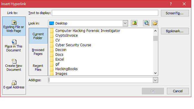
Insert Hyperlink dialogue box will appear. Now, to create a link to an already created Excel file, select a file.
Now, to create a link to a web page, type the text to display, and click OK. We have entered google.com as text to display and the following image is showing us the result.
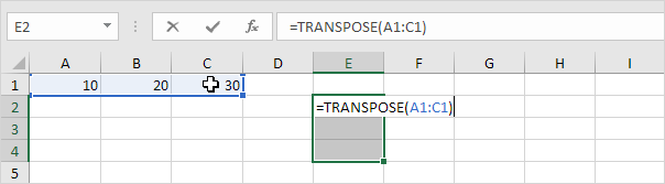
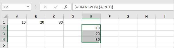
15. Transpose
The TRANSPOSE function allows users to a transposed range of cells. It returns a horizontal range of cells when a vertical range is entered as an input. Or a vertical range of cells is returned if a horizontal range of cells is entered as an input. It comes under a Lookup/Reference Function of features of MS Excel.
Syntax: TRANSPOSE( range )
After entering the function. The below image is showing us the result.
Check this article as a VIDEO
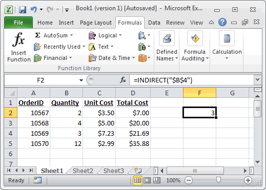
16. INDIRECT
This function returns the reference to a cell based on its string description. It comes under the Lookup/Reference feature of MS Excel. It returns the referenced cell’s value.
Syntax: INDIRECT( string_reference, [ref_style] )
The following image shows us the use of the INDIRECT function.
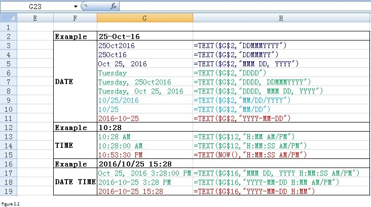
17. FORMAT
FORMAT function accepts a string argument and returns it as a formatted string. It comes under the String/Text Function of Microsoft Excel.
Syntax: Format ( expression, [ format ] )
Let’s look at some Excel FORMAT function examples:
The above figure shows us the use of the Format function.
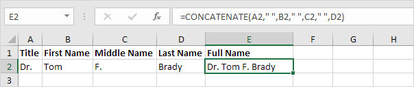
18. CONCATENATE
CONCATENATE function enables users to join 2 or more strings together.
The following figure is showing us the use of the CONCATENATE function:
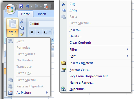
19. Paste Special
Paste Special is one of the most amazing features of Excel. It enables the user to control how the content will be displayed when pasted from the clipboard. The following image is showing how to use paste special.
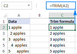
20. TRIM
If you want to remove extra spaces from a spreadsheet then the TRIM function is useful. The trim function will remove all the unnecessary trailing and leading spaces from the cell.
Syntax: TRIM(text)
The above figure is showing you how the TRIM function works. It has removed the unwanted spaces from column A and the result is displayed in column C.
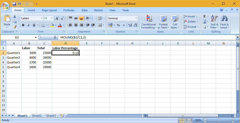
This is one of the coolest Microsoft Excel features. The round function is utilized to receive an amount that has several decimals and round it to the number of specified decimals.
The following image is displaying the use of the Round function. In this, we have divided labor into Total expenses in column D. If we just implement the formula B2/C2, the large number after the decimal will be displayed.
To avoid this we have used the Formula: =ROUND(B2/C2,2). This will format the cell into 2 decimals and it will display it perfectly. The Round() function is pretty useful if there are large decimal numbers. This function is similar to that of Round() function used in SQL.
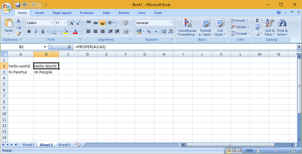
22. PROPER
The PROPER function is used to make each of the entered phrases into a proper-looking style or sentence cases. It is a text function that is used to capitalize each word. The following image is displaying the use of the PROPER function. In this function, you just have to enter the formula =PROPER(A2:A3). The range can be anything. The function is a string function and will convert the entered text into the proper sentence case. The PROPER function is crucial if users have involved in text spreadsheets while data migration. It is simple to implement and use to convert text into proper sentence structure.
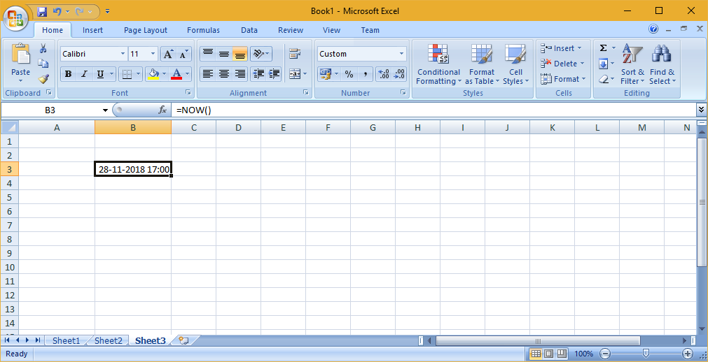
23. NOW function
The NOW function is pretty simple. It is an uncomplicated function that will just tell users precisely what time and day it is. By using this function users can format it as a date to show the date and time or just the date. The following image is displaying the use of NOW() function. Cell B3 is displaying the current date of your system after you enter this formula =NOW() in cell B3.
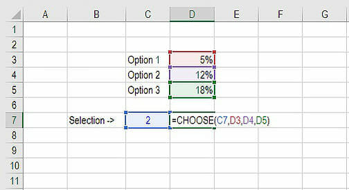
24. CHOOSE function
The CHOOSE function is excellent for summary analysis in commercial modeling. It enables users to choose between a particular number of options, and answer the selected choice. For example, there are three distinct postulates for revenue growth next year: 5%, 12%, and 18%. Applying the CHOOSE formula users can return 12% if they recognize Excel you want choice. The following image is displaying the result.
25. Named Ranges
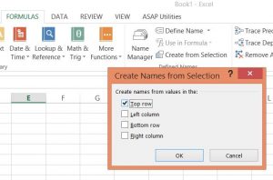
This is one of the best advanced Excel features. If there are large numbers then this feature is helpful to give names to ranges so that users can refer to these names in advanced Excel formulas without clicking and picking long ranges. To promptly give names to the ranges follow these steps:
Click on the Formulas menu option on the ribbon.
Now in the next step, click on the Create from Selection button.
Now in the third step, Select the ranges to give names.
The following image is displaying the use of Named Ranges.
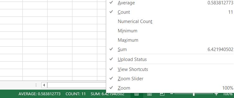
26. Quick Feature
This is one of the best advanced excel tools for business. This feature gives aggregate statistics like Average, Count, Numerical Count, Max, Min, and Sum of the data from a picked range without inserting any formula. To display these results in the bottom toolbar, right-click on the toolbar and pick the wanted statistic. The following image is displaying the use of this feature. The quick feature is really helpful if users want to aggregate numbers quickly.
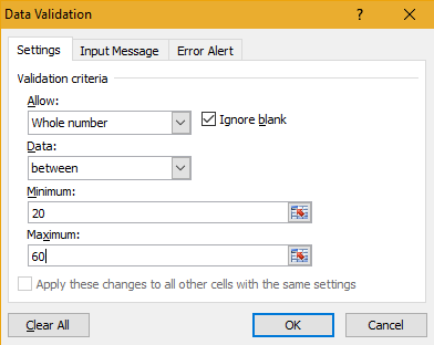
27. Input Restriction
This feature is useful to preserve the validity of data. Often, users need to check the input value and give some advice for further steps. For example, the date of birth in the sheet should be in DD/MM/YYYY format and all users engaging should be between 18 and 55 years old. This feature is just like constraints.
To assure that data outside of this rule isn’t inserted, go to Data->Data Validation->Setting, input the conditions and shift to Input Message to give suggestions like, “Please input your date of birth in DD/MM/YYYY format, which should range from 20 to 60. Users will get this message when hovering over the pointer in this area and get a notification message if the entered data is not proper. The following image is displaying the use of these features.
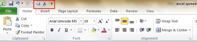
28. New Shortcut Menu
Usually, there are three shortcuts on the top menu. These are Save, Undo Typing, and Repeat Typing. Nevertheless, if users want to apply or use more shortcut options such as Copy and Cut then they can set them up by following these steps: File->Options->Quick Access Toolbar, add Cut and Copy from the left column to the right, save it. The two more shortcuts will get added to the top menu. This is one of the coolest features of Excel which helps users to quickly apply Excel useful functions. There are many such functions that can be implemented on the top menu by following this simple trick.
29. Hide Data
Almost all Excel enthusiasts understand how to hide data by right-clicking to select the Hide function. The problem with this is that this can be quickly seen if there is only limited data. The safest and smoothest way to hide data completely is to utilize the Format Cells function. Follow these steps: Pick the area and go to Home->Font->Open Format Cells->Number Tab->Custom-> Type;;; -> Click OK, then all the contents in the area will be hidden, and can only be spotted in the preview area near to the Function button.
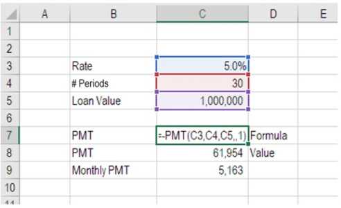
30. PMT and IPMT
If users are working in any finance sector, real estate, FP&A, or any business analyst position that handles debt programs then these ones are one of the most important Excel advanced functions. The PMT formula provides users with the value of equal amounts over the period of a loan. Users can apply it in combination with IPMT which explains to users the interest amounts for the equivalent type of loan and then separates principal and interest amounts. The following image is displaying how to use the PMT function to get the regular mortgage amount for a $1 million debt at 5% for 30 years.
31. REPT()
The REPT Function is classified under logical functions. The function will duplicate characters a supplied number of times. In a business report, REPT can be used to load a cell to a particular range. We can also develop histograms, a chart usually applied in commercial modeling, utilizing the function by altering values immediately into a definite number of (iterated) cases. This is one of the most important excel functions. It is widely used in business analytics.
Formula =REPT(text, number_times)
The following sample returns the string in the column, [MyValue], returned for the number of terms in the column, [MyAmount]. Because the method continues for the complete column, the output string depends on the topic and amount value in every row.
=REPT([MyValue],[MyAmount])
Output
MyValue
MyAmount
ResultingColumn1
Text
3
TextTextText
Number
0
89
3
898989
32. CONCATENATEX
This function Concatenates the outcome of the character assessed for each row in a table. This function accepts as its primary parameter a table or that delivers a table. The second parameter is a column that includes the conditions you want to concatenate, or a character that reflects value. Example
EMP table
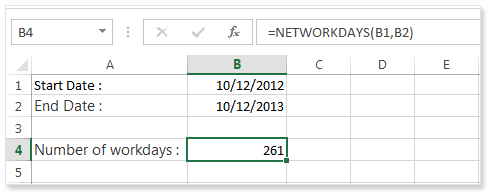
The NETWORKDAYS function estimates the number of workdays between two terms in Excel. It also enables you to jump-defined leaves and only includes working days. It is characterized in Excel as a Date/Time Function. You can apply this method to determine working days in Excel within two dates.
Formula
=NETWORKDAYS(start_date, end_date, [holidays])
For example, the example below gives the number of workdays between the beginning (10/10/2012) and end date (12/10/2013).
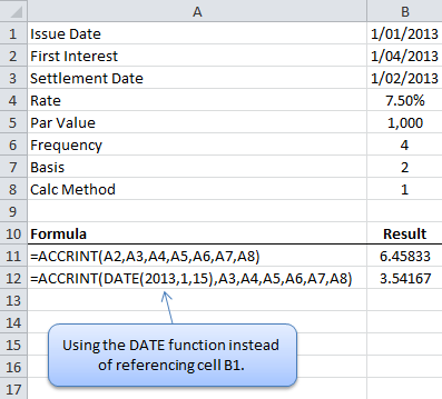
34. ACCRINT
The ACCRINT function will determine the accrued profit for a bond that gives interest periodically. ACCRINT assists users to determine the accrued benefit on security, such as a bond, when that security is traded or is transported to a new buyer on a date other than the delivery date.
The ACCRINT function was included in MS Excel 2007 and so is not accessible in earlier versions. In economics, security rates are rated “clean”. The “clean price” of a bond eliminates any profit collected since the delivery date or most current card payment. The “dirty price” of a security is the amount including accrued gain. The ACCRINT function can be applied to determine accrued benefit for security that gives periodical business but pay heed to date arrangement.
The following image is displaying the use of ACCRINT
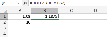
35. DOLLARDE
It assists in transforming a dollar amount in partial representation into a dollar value shown in decimal representation. DOLLARDE will break the section part of the content by an integer defined by the user. It is utilized in valuing US depository bond quotes, which are assessed to the most next 1/32 of a dollar. The function is very helpful for business analysts when creating business reports using capital market figures, as divided dollars are utilized for bond prices. DOLLARDE is accessible from MS Excel 2007.
Formula
=DOLLARDE(fractional_dollar, fraction)
The following image is displaying the use of DOLLARDE function
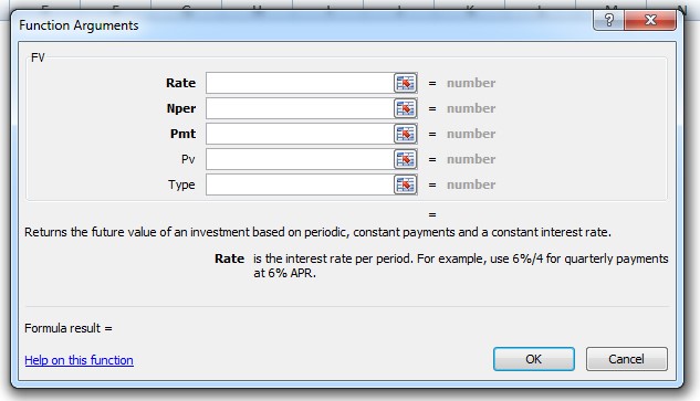
36. FV
The FV function in Excel is a business function that gives the expected value of an investment. You can apply the FV function to obtain the anticipated price of an investment considering intermittent, regular payments with a fixed interest rate. Users should be constant about the units they apply for defining valuation and nper. If you make regular returns on a four-year loan at 12% yearly interest, one can apply 12%/12 for valuation and 4*12 for nper.
=FV (rate, nper, pmt, [pv], [type])
Example: Take the sample data in the given table given in Microsoft, and paste it in cell A1 of your worksheet. For functions to display results, choose them, press F2, and then Enter.
Data
Description
0.06
Interest rate
10
Total payments
-200
Amount
-500
Present value
1
Due Payment is due at the beginning of the period
Formula
Description
Result
=FV(A2/12, A3, A4, A5, A6)
Future value of an investment using the terms in A2:A5.
$2,581.40
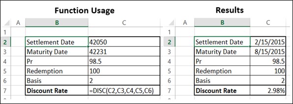
37. DISC function
The DISC function determines the Discount Rate for security. The security’s adjustment date or one can say that the date that the security ticket is bought. The security’s maturity date or the date that the security ticket expires
Example: The following image is displaying the use of the DISC function.
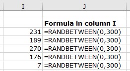
38. RANDBETWEEN
This function allows users to pick a number within an already defined range of numbers. Once users place the lowest and the highest numbers, Excel can pick the correct information from the areas to which the titles in the Range are connected and select from them. The syntax of this function is:
=RANDBETWEEN(starting point, ending point)
Example:
The Randbetween function is used to generate one or multiple random numbers between two values.
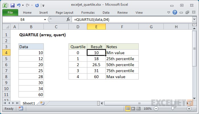
39. QUARTILE
The Quartile function gives the quartile or each of four equal groups in a distributed assortment of data and can give minimum value, first quartile, second quartile, and maximum value. This function returns the quartile value of the cells in an arrangement. It also returns a statistical value as per the entered percentile. Quartiles usually are applied in sales and review data to classify communities into groups. For instance, one can apply the QUARTILE function to discover the top 25 percent of revenues in a population.
Syntax:
=QUARTILE (array, quart)
Example:
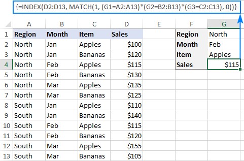
40. INDEX MATCH
An index match function is an exceptional option for the VLOOKUP or HLOOKUP formula that has some disadvantages for implementing lookup jobs. The INDEX MATCH is a sequencing method with 2 distinct functions. For instance, when you are viewing and giving someone’s height based on their identity or name, you can apply this function to switch both the variables applying the INDEX MATCH.
For example, here we want to get the sales amount for a specific item in a particular area and month. The function is a high-level version and gives the output, a match based on a particular pattern. To assess various measures, we apply the multiplication process that serves as the AND operator.
About the Author
ByteScout Team of WritersByteScout has a team of professional writers proficient in different technical topics. We select the best writers to cover interesting and trending topics for our readers. We love developers and we hope our articles help you learn about programming and programmers.
Internationalization aka i18n is a concept that refers to the development of user interfaces in different languages. The major benefit of supporting multiple languages is...
1. What is a Spring framework? Spring is an amazing open-source software program application machine made to lower the intricacy of big business enterprise software...