Our ByteScout SDK products are sunsetting as we focus on expanding new solutions.
Learn More
Important Update
ByteScout SDK Sunsetting Notice
Our ByteScout SDK products are sunsetting as we focus on our new & improved solutions.Thank you for being part of our journey, and we look forward to supporting you in this next chapter!
We start from the general description of regression models and examine bias and variance concepts. Then we explain Lasso and Ridge regressions by demonstrating their Python implementations. In the last part, we summarize the tutorial and discuss the difference between the methods we reviewed.
Regression Models
Regression models are methods of estimating the dependent variables using independent variables. The simplest one is Linear regression which estimates the output by establishing a linear relationship between independent inputs.
Y= Xβ + ε
ε ∼ N(0,σ^2)
The Y’s here are independent random variables, and X’s are linear combinations of a certain number of variables. ε are also random variables and represent the unobservable error which comes from the normal distribution with mean 0 and variance 〖σ_ 〗^2. Our goal is to estimate the unknown β parameters. We can estimate β, by minimizing the loss function using the maximum likelihood estimators or the Ordinary Least Squares(OLS) method.
This equation shows minimizing the sum of the squares of the difference between real output values (y) and the estimated ones with the regression curve we constructed (Xβ) (i.e. the error value).
Bias and Variance Terms
Bias is the difference between the estimated and real output value. If our model has a high bias, it will oversimplify the training data. This causes high errors in our training and test data.
Variance is a value that declares the spread of our data for a given data point. If our model has high variance, it fits the training set more than enough. It memorizes the observations instead of finding a pattern that can generalize the previously observed testing set. This causes low errors in the training set but high errors in the testing set.
We minimize our loss function in machine learning by fitting the model to the data. If the loss function is too close to 0, our model might be overtrained; if it is far from 0, there is the possibility of under-fitting, which refers to insufficient learning. In other words, if the model starts to memorize the observations instead of discovering the pattern in the data, the estimated values will be very close to the real output values so the loss function will decrease.
The complexity of the model increases with the number of parameters. When the model’s complexity increases, it will have high variance and low bias. It will have a high bias in low complexity, and low variance since OLS takes care of all variables equally and unbiased. The complexity increases when adding new variables to the model.
Gauss-Markov Theorem proves that the OLS estimator is the Best Linear Unutral Estimator for the linear regression models. In this definition, Linearity refers to the dependent variable (Y) of the model is a linear function of a random variable. Unbiased means that the model has zero bias for all values of parameters. OLS is the best estimator with the lowest variance amongst the linear unbiased estimators.
Ridge and Lasso’s regressions are two different techniques that can reduce the model’s complexity and prevent overfitting.
Lasso Regression and Python Implementation
Lasso regression uses the L1 penalty given below to prevent overfitting. Here t is a parameter that refers to the degree of the regularisation.
For some t>0 ,∑_(j=0)^p |(β_j ) ̂ | ≤ t
Lasso regression completely ignores some attributes because it uses L1 regularization (i.e. it takes the coefficients’ absolute value instead of squaring them). So Lasso regression plays an important role also in feature selection.
# we import necessary libraries and functions
import matplotlib.pyplot as plt
from sklearn.linear_model import LinearRegression
from sklearn.linear_model import Ridge
from sklearn.linear_model import Lasso
from sklearn.model_selection import train_test_split

# first we load boston data and divide it into training and testing sets
X, y =load_boston(return_X_y=True)
X_train, X_test, y_train, y_test = train_test_split(X, y, test_size=0.3, random_state=3)

# we define an ordinary linear regression model (OLS)
linearModel=LinearRegression()
linearModel.fit(X_train, y_train)

# evaluating the model on training and testing sets
linear_model_train_r2=linearModel.score(X_train, y_train) # returns the r square value of the training set
linear_model_test_r2=linearModel.score(X_test, y_test)
print('Linear model training set r^2..:', linear_model_train_r2)
print('Lineer model testing r^2..:', linear_model_test_r2)

# here we define a Lasso regression model with lambda(alpha)=0.01
lasso=Lasso(alpha=0.01) # lasso has the probability of equalizing the beta values to 0
lasso.fit(X_train, y_train)
lasso_train_r2=lasso.score(X_train, y_train)
lasso_test_r2=lasso.score(X_test, y_test)
print('Lasso model (alpha=0.01) train r^2..:', lasso_train_r2)
print('Lasso model (alpha=0.01) test r^2..:', lasso_test_r2)

# we define another Lasso regression model with lambda(alpha)=1
lasso2=Lasso(alpha=1)
lasso2.fit(X_train, y_train)
lasso2_train_r2=lasso2.score(X_train, y_train)
lasso2_test_r2=lasso2.score(X_test, y_test)
print('Lasso model (alpha=1) train r^2..:', lasso2_train_r2)
print('Lasso model (alpha=1) test r^2..:', lasso2_test_r2)

# another Lasso regression model with lambda(alpha)=100
lasso3=Lasso(alpha=100)
lasso3.fit(X_train, y_train)
lasso3_train_r2=lasso3.score(X_train, y_train)
lasso3_test_r2=lasso3.score(X_test, y_test)
print('Lasso model (alpha=100) train r^2..:', lasso3_train_r2)
print('Lasso model (alpha=100) test r^2..:', lasso3_test_r2)

# visualize the values of the beta parameters
plt.figure(figsize=(8,6))
plt.plot(lasso.coef_, alpha=0.7, linestyle='none', marker='*', markersize=15, color='red', label=r'Lasso: $\lambda=0.01$')
plt.plot(lasso2.coef_, alpha=0.7, linestyle='none', marker='d', markersize=15, color='blue', label=r'Lasso: $\lambda=1$')
plt.plot(lasso3.coef_, alpha=0.7, linestyle='none', marker='o', markersize=15, color='green', label=r'Lasso: $\lambda=100$')
plt.plot(lineerModel.coef_, alpha=0.7, linestyle='none', marker='v', markersize=15, color='orange', label=r'Linear Model')
plt.xlabel('Attributes', fontsize=16)
plt.ylabel('Attribute parameters', fontsize=16)
plt.legend(fontsize=16, loc=4)
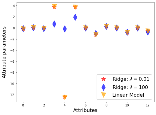
Ridge Regression and Python Implementation
Ridge regression tries to find β ̂ parameters with the smallest variance, compromising the concept of unbiasedness.
Ridge regression is a regression variant using L2 regularization, shown below.
〖|(|β ̂ |)|_2〗^ =√(〖β_0〗^2+〖β_1〗^2+…+〖β_p〗^2 )
As we see in the formula below, L2 penalty (λ〖|(|β ̂ |)|_2〗^2 ) takes the square of the parameters. All weights are equally reduced towards 0. The λ parameter determines the degree of regularization. When λ→0, the cost function transforms into the least-squares method’s cost function. Various methods can be used to find this parameter. The most used methods for finding optimal λ are finding the value that minimizes the Mean Square Error(MSE) of the model at various values using the cross-validation or looking for the best R^2 score.
# we import necessary libraries and functions
import matplotlib.pyplot as plt
from sklearn.linear_model import LinearRegression
from sklearn.linear_model import Ridge
from sklearn.linear_model import Lasso
from sklearn.model_selection import train_test_split

# first we load boston data and divide it into training and testing sets
X, y =load_boston(return_X_y=True)
X_train, X_test, y_train, y_test = train_test_split(X, y, test_size=0.3, random_state=3)

# we define an ordinary linear regression model (OLS)
linearModel=LinearRegression()
linearModel.fit(X_train, y_train)

# evaluating the model on training and testing sets
linear_model_train_r2=linearModel.score(X_train, y_train) # returns the r square value of the training set
linear_model_test_r2=linearModel.score(X_test, y_test)
print('Linear model training set r^2..:', linear_model_train_r2)
print('Lineer model testing r^2..:', linear_model_test_r2)

# here we define a Ridge regression model with lambda(alpha)=0.01
ridge=Ridge(alpha=0.01) # low alpha means low penalty
ridge.fit(X_train, y_train)
ridge_train_r2=ridge.score(X_train, y_train)
ridge_test_r2=ridge.score(X_test, y_test)
print('Ridge model (alpha=0.01) train r^2..:', ridge_train_r2)
print('Ridge model (alpha=0.01) test r^2..:', ridge_test_r2)

# we define a another Ridge regression model with lambda(alpha)=100
ridge2=Ridge(alpha=100) # when we increase alpha, model can not learn the data because of the low variance
ridge2.fit(X_train, y_train)
ridge2_train_r2=ridge2.score(X_train, y_train)
ridge2_test_r2=ridge2.score(X_test, y_test)
print('Ridge model (alpha=100) train r^2..:', ridge2_train_r2)
print('Ridge model (alpha=100) test r^2..:', ridge2_test_r2)

# visualize the values of the beta parameters
plt.figure(figsize=(8,6))
plt.plot(ridge.coef_, alpha=0.7, linestyle='none', marker='*', markersize=15, color='red', label=r'Ridge: $\lambda=0.01$')
plt.plot(ridge2.coef_, alpha=0.7, linestyle='none', marker='d', markersize=15, color='blue', label=r'Ridge: $\lambda=100$')
plt.plot(linearModel.coef_, alpha=0.7, linestyle='none', marker='v', markersize=15, color='orange', label=r'Linear Model')
plt.xlabel('Attributes', fontsize=16)
plt.ylabel('Attribute parameters', fontsize=16)
plt.legend(fontsize=16, loc=4)
Summary and Discussion
Overfitting and underfitting are prevalent situations while we train machine learning models. Overfitting refers to the increasing error rates for the samples in the testing set due to memorizing the samples in the model’s training. Underfitting refers to high error rates due to insufficient training samples’ modeling.
In this tutorial, we started with the basic concepts of linear regression and included the mathematics and Python implementation of Lasso and Ridge regressions, which are recommended to avoid overfitting. Lasso regression uses the L1 norm, and therefore it can set the beta coefficients(weights of the attributes) to 0. Ridge regression uses L2 norm regularization, and so the coefficients might be very low but not 0. You can observe this by running the code snippet below.
As you can see in the Ridge regression, the number of attributes has not decreased. However, as the alpha parameter increased in the Lasso regression, our number of features decreased. In other words, as we mentioned in our article, Lasso regression makes feature selection. In the Lasso regression, when we give high alphas, our scores were low because it did a significant number of attribute eliminations, and this caused underfitting. In overfitting, we increase the alpha and reduce the effect of overfitting, against in case of underfitting, we decrease the alpha parameter. We see that shrinking the alpha parameter too much brings us closer to the linear regression score.
About the Author
ByteScout Team of WritersByteScout has a team of professional writers proficient in different technical topics. We select the best writers to cover interesting and trending topics for our readers. We love developers and we hope our articles help you learn about programming and programmers.
PDF or Portable Document Format files are immensely popular among every individual, irrespective of the profession. This popularity is due to its ability to capture...