AI Functions Cheat Sheet for Developers

Cheatsheets are great. They provide tons of information without any fluff. So today we present you a small cheat sheet consisting of most of the important formulas and topics of AI and ML. Towards our first topic then.

Table of content

• Activation functions
• Loss functions
  • Regression Loss Function
  • Classification Loss Function
  • Statistical Learning
  • Statistical Inference
    • Regression
    • Classification
    • Feature Reduction

Activation functions

Activation functions are kind of like a digital switch that controls whether a specific node (a neuron) in a neural network would ‘fire’ or not. Following are the most commonly used ones:

1. Sigmoid:

The sigmoid (aka the logistic function) has a characteristic ‘S’ shape. One of the main reasons why it’s used widely is because the output of the function (range) is always bounded by 0 and 1. The function is differentiable and monotonic in nature. This activation function is used when the output is expected to be a probability. The function is given by,

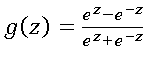
2. Tanh:

Tanh function (aka the hyperbolic tangent function) is similar to Sigmoid in the sense that it also has the characteristic ‘S’ shape. But the main difference between the Sigmoid and Tanh is that the range of Tanh is bounded by -1 and 1, whereas the range of Sigmoid is bounded by 0 and 1. The function is differentiable and monotonic in nature. The function is given by,

3. ReLU:

The ReLU (Rectified Linear Unit) is debatably the most widely used activation function. It’s also known as a ramp function. Unlike Sigmoid or Tanh, ReLU is not a smooth function, i.e. it is not differentiable at 0. The range of the function is bounded by 0 and infinity. The function is monotonic and unbounded in nature. The function is defined as,

4. Leaky ReLU:

Leaky ReLU is a specific version of the ReLU activation function. Leaky ReLU is primarily used to address the ‘Dying ReLU’ problem. The small epsilon value converts the range of the function from (0, infinity) to (-infinity, infinity). Like ReLU, Leaky ReLU is monotonic in nature. The function is given by,  with ϵ≪1.

Loss functions

Roughly speaking, loss functions define how good a prediction is. Given the true value and the predicted value, the loss function gives an output that is congruent to the ‘goodness’ of the prediction.

Depending on the type of the task at hand, the loss functions can be broadly divided into 2 categories: regression loss functions, and classification loss functions.

Regression Loss Function

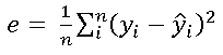
1. Mean Square Error:

Mean squared error (also known as the MSE, the quadratic Loss, and the L2 Loss) is a measure that defines the goodness in terms of the squared difference between the true value and the predicted value. Due to the nature of the function, the predictions that are far from the actual values are penalized much more severely compared to the values that are somewhat closer. The loss is given by,

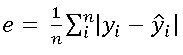
2. Mean Absolute Error:

Mean absolute error (or L1 error) is a measure that defines the goodness of the predicted value in terms of the absolute difference between the actual value and the predicted value.  As it does not square the differences like MSE it is much more robust to the outliers. The formula is given by,

Classification Loss Function

1. Cross-Entropy Loss:

Cross entropy loss is the most common type of loss function for classification problems. Thanks to its definition, it’s also called the negative log-likelihood error. The characteristic of the cross-entropy loss is that it heavily penalizes the predictions that are both confident and wrong. The loss function is given by,

2. Hinge Loss:

Living in the SVMland, Hinge loss is something that you would not come across a lot. In simple terms, the score of the correct class should be greater than the cumulative score of all the other classes by some margin. It’s used for maximum margin classification in the support vector machines. The loss function is defined as follows:

Statistical Learning

The whole statistical learning domain could be divided into 3 categories:

1. Supervised learning: Both the input data and the labels are available for the training data.
2. Unsupervised learning: Only the input data is available.
3. Reinforcement learning: The input data and an interactive environment (with which the agent can interact) are available.

Statistical Inference

The machine learning tasks can be divided into 3 categories – regression, classification, and feature reduction.

Regression

Given the training data, the regression task needs you to predict the value of some input features. The point to note here is that the predicted value can numerically be anything.

1. Linear: One of the simplest models for regression is the linear model. The linear models, having a low variance, often suffer from high bias.
2. Logistic: Logistic regression is the preferred method for many binary classification problems where you would want a lightweight model. It uses the earlier mentioned Sigmoid function as activation. It again suffers from high bias while having low variance.

Classification

Given the training data, the classification needs you to assign a feature of value from some predefined values.

1. Neural network: It tries to come up with a model that is a combination of linear and non-linear actions. Overfitting, in general, is a big problem in neural networks.
2. Naive Bayes: Uses the principle of probability and the maximum likelihood estimates of the data point for prediction. Known to work great for natural language processing.
3. Support Vector Machine: The support vector machine is a class of classifiers that are used heavily for binary classification problems. The SVM aims to come up with a maximum-margin separator for the given data points. SVMs have low bias but exhibit high variance.
4. K-Nearest Neighbours: A model that is used for nothing other than baseline testing these days. Uses the proximity of the data points for prediction.

Feature Reduction

Oftentimes your data would have way too many features than you might like. Additionally, more features imply more complex models, which in turn imply lower speed and accuracy. So reducing the number of features in a meaningful way is almost always a good idea.

1. Principal Component Analysis: Principal component analysis (PCA) helps distill the feature space into so-called principal components that describe the highest variance. It’s almost always a good idea to apply it to high-dimensional data.

   

About the Author

ByteScout Team of Writers ByteScout has a team of professional writers proficient in different technical topics. We select the best writers to cover interesting and trending topics for our readers. We love developers and we hope our articles help you learn about programming and programmers.