Home
/
Blog
/
Ultimate Exploration of Deep Sql Queries and Examples

Ultimate Exploration of Deep Sql Queries and Examples

The power and functionality of SQL database programming are immense! But this can only be seen in the relational JOIN operations which connect a set of tables with a purpose. JOIN statements enable us to find conditional relationships within tables or datasets. We can then do calculations, sort, and even create new tables based on relationships established among key fields!

Moreover, many tutorials simply illustrate the syntax of SQL statements without deeply exploring how they are used. SQL is simple in form, but it gives us rich possibilities to express subtle and ingenious patterns in data. In this Bytescout deep SQL tutorial, we will look at an actual sales database. First, we will define a set of tables with primary keys. Then build JOINs and explore the interesting Views which arise from our relational SQL database example.

We will go beyond the function of the language and provide you with a real-world database. What we have in mind here is an advanced SQL tutorial with examples. We will join our customer, product, and sales tables and use complex SQL query examples to answer these questions:

Which products did a particular customer purchase?
What are our best-selling products?
Which months had the highest sales…
Which of our customers did not make purchases in March?

As you can see, it’s possible to get a plethora of useful data when the tables are built and organized correctly. The next step is to learn how to use inner and outer JOINS with multiple tables.

SQL code examples and SQL query examples, as well as SQL subquery examples, will follow naturally. This will be a companion article to our popular, “Ultimate List Of 40 Important SQL Queries.” Many of the queries in that list will now contain links to “explore in-depth” linking to their use in this real-world example.

Setting up a table for the database

CREATE TABLE Customer (
Customer ID varchar(80),
Firstname varchar(80),
Lastname varchar(20),
);

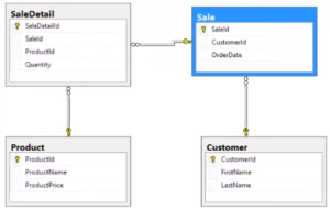
Go ahead and replicate the above CREATE TABLE statement with the other names in the diagram below to create tables in your own DB. To follow the subsequent examples, make your tables similar to those in the following diagram:

Add Database Structure

Now that we have our tables, let’s add structure by first defining the PRIMARY KEY fields in each table. Primary keys are essential to the relational aspect of a database. Primary key fields guarantee that JOIN statements will maintain data integrity. A Primary Key column may contain only unique values, no duplicates. Accurate DB indexing also depends on primary keys. Here’s how to add a primary key:

CREATE TABLE Customer (
CustomerID int NOT NULL 
...
PRIMARY KEY (CustomerID )
);

If you have already created all the tables above, you can change the necessary fields to primary keys with these statements:

ALTER TABLE CustomerID
ADD CONSTRAINT CustomerID PRIMARY KEY (CustomerID)

Primary and Foreign Keys Enforce Our Data Model

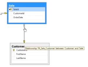
Have a look a the diagram of our four tables above. Notice that all the tables have primary keys defined. Some tables also have “foreign keys.” Foreign key relationships prevent one table from having data that does not have a match in another table. As shown in the next diagram, we cannot have a sale without a valid customer:

Add data columns

If you need to add more data columns to a table that you’ve already added to the DB, use the ALTER TABLE statement. For example, you might decide to send a happy birthday email to your customers. You can do so with this line of code:

ALTER TABLE Customer ADD Birthday varchar(80)

Later, you can add a SELECT query to produce a report which shows all your customers who have birthdays coming up in the next week, and even write a script to auto-generate an email to send them a happy birthday message!

Retrieving Tables and Building Results

Now we have built a sample database that is simple but effective for demonstrating the most powerful features of SQL commands with syntax and examples. The first step is to use the all-important SELECT statement to gather the exact data we need for queries.

The data returned from SELECT statements is stored in result tables called the “result-set.” In the example below, column1, column2, etc. are the field names of the table we want to get data from. To select all the fields available in the table use the “*.” When a table contains many columns of data that are not relevant to a JOIN, you can optimize the result set by only including necessary columns like this:

SELECT column1, column2, ...FROM table_name;

To get a result-set including all fields from all our tables, we enter the following SELECT commands using the “*” in this way:

SELECT * FROM Customer;
SELECT * FROM Product;
SELECT * FROM Sale;
SELECT * FROM SaleDetail;

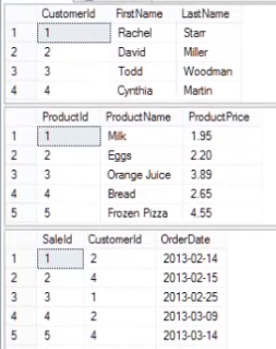
And now in this diagram, we have some example data in each table. We will use this sample data to illustrate the results of queries and calculations:

We have a total of four tables (above and below diagrams). Notice that each sale row in the Sale table has a CustomerID to identify who ordered the product…

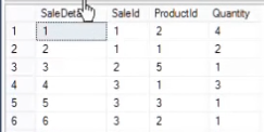
And notice that each SaleDetail row has both a SaleID, one for each transaction, and a ProductID, each of which points to inventory items bought in the sale. So, a unique customer in each sale transaction can buy various products. And the rules are enforced by the structure we’ve created in our DB! By building our tables in this intelligent way, we can use all the power of SQL to create meaningful query results, such as inventory and sales reports! Also, this will enable us to learn SQL programming by example.

Introducing the Ultimate Interface: The JOIN statement

The best SQL query examples rely on JOIN statements to establish relationships among tables. We group and separate data meaningfully into distinct tables in order to have the greatest flexibility in querying the data. The JOIN statement is the core component of SQL that creates the interfaces between tables. We’ll begin with the INNER JOIN:

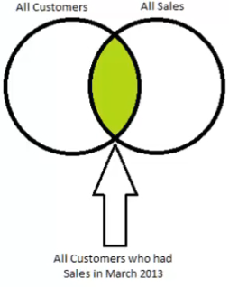
Suppose we want to query our DB for all customers who had made purchases in the month of March 2013. We can write a query using the INNER JOIN to connect our tables accordingly. As shown in the diagram above, the INNER JOIN will create a query that returns the intersection of the Customer and Sale tables as a result-set. Here’s how to do it:

SELECT Customer.CustomerId FROM Customer
INNER JOIN Sale on
Customer.CustomerId = Sale.CustomerId;

This SELECT query will give us a result-set including the sales of all customers. Now, we want to further refine this query to include only sales that occurred in the month of March 2013. To do this we add the WHERE clause.

Adding the WHERE clause

The WHERE clause is a very powerful conditional operation in SQL programming, and we will make extensive use of it. Let’s see an example to refine our INNER JOIN to include only sales in the month of March 2013. Here’s how to write the SELECT query with a WHERE clause:

SELECT DISTINCT Customer.CustomerId FROM Customer
INNER JOIN Sale on
Customer.CustomerId = Sale.CustomerId
WHERE Sale.OrderDate BETWEEN '3/1/2013' AND '3/31/2013'

Notice that BETWEEN clause is a very convenient way of writing “greater than or equal to” or “less than or equal to” operators from other languages. And also notice the OOP style notation of referring to the CustomerID field, which can be used conveniently to distinguish it in tables containing a field of the same name:

Customer.CustomerId = Sale.CustomerId

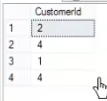
Now the result-set of the WHERE clause above is a simplistic view like this:

But this is a very useful result that can be used to create still more interesting outcomes.

Including more elements

We can further narrow the result-set to include, for example, a list that shows each customer only once. In other words, we can use the DISTINCT clause to show each customer only once:

SELECT DISTINCT Customer.CustomerId FROM Customer
INNER JOIN Sale on
Customer.CustomerId = Sale.CustomerId
WHERE Sale.OrderDate BETWEEN '3/1/2013' AND '3/31/2013'

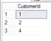
After adding the DISTINCT clause, notice that the above result-set is reduced accordingly:

Reducing Verbosity with Shortcuts: Alias

Adding shortcuts

In fact, we can add several notation shortcuts to reduce the verbosity of the SQL code. When defining table names, we only need to use the table name once, followed by the alias name, in this case, “c.”Also, because the INNER JOIN is the default type, the keyword “INNER” is optional and can be omitted. Then the above SELECT query becomes:

SELECT DISTINCT c.CustomerId FROM Customer c
INNER JOIN Sale s on
c.CustomerId = s.CustomerId
JOIN SaleDetail sd ON
s.SaleId = sd.SaleId
WHERE s.OrderDate BETWEEN '3/1/2013' AND '3/31/2013'

Here we have the same result-set as above, but with reduced code verbosity. Remember to make your alias names meaningful, so that other developers can read your algorithms!

JOIN Queries for Multiple Tables

We can use JOIN to create interfaces and relationships for multiple tables. Let’s look at an example that connects ALL the tables in our example database above. We want to produce a sales report for the month of March, and so we need to get data from all resources at once.

Remember that we can only JOIN tables that have common fields. In the first JOIN below, we connect the Customer and Sale tables on their common field name:

SELECT c.FirstName, c.LastName, s.OrderDate, p.ProductName, sd.Quantity, sd.Quantity * p.ProductPrice AS TotalPrice  FROM Customer c
INNER JOIN Sale s on
c.CustomerId = s.CustomerId
JOIN SaleDetail sd ON
s.SaleId = sd.SaleId
JOIN Product p
on sd.ProductId = p.ProductId
WHERE s.OrderDate BETWEEN '3/1/2013' AND '3/31/2013'

We specified all the data fields we want in the first line. Notice that the fields specified to come from the tables in the subsequent JOINs. For example, sd.Quantity comes from the SaleDetail table which is aliased “sd.” So, there are a total of three JOINs to connect our four tables. Let’s discuss how these JOINs work together, and the result-set we get as an outcome.

As mentioned, we are creating a sales report for the month of March 2013. We will need for our report details including the customer name, and a list of their purchases. This is added by the first JOIN. Each sale contains a list of products purchased in the transaction. We obtain this detail by JOINing the Sale table with the SaleDetail table in the second JOIN.

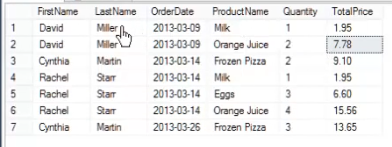
Finally, we want to list the products and prices sold in each transaction. This we accomplished by JOINing the SaleDetail to the Product table, which contains item description and pricing info. This is added by the third JOIN. And here is the result-set from our sales report query:

This single query reveals a lot of the power of SQL to gather, filter, sort, and calculate on tables in a very fast and efficient way. In effect, we produced a sales report for the month of March which breaks out all the details of all transactions. It shows customer name, transaction date, products, quantities, and prices of items sold! This is the best demo of SQL fundamentals.

Because the INNER JOIN represents the intersection of one or a group of tables, it is the most frequently used of all JOIN statements. However, there are many other JOIN types that produce unique result sets. Here is a list of a few others:

LEFT JOIN – All records from the left table and any right matches
RIGHT JOIN – All records from the right table and any left matches
FULL JOIN – All records when either left or right matches
SELF JOIN – Compares records within the same table

The SELF JOIN is also frequently useful. We can use the SELF JOIN to find customers who live in the same city, for example:

SELECT C.FirstName AS name, C.City
FROM Customer C, Customer B
WHERE C.CustomerID <> B.CustomerID
AND C.City = B.City
ORDER BY C.City;

As you can see, this is a very convenient way to analyze data within a single table. The same table is given two different aliases for this purpose. The result-set will contain all customers from a single table who have the same value in the City field.

Calculating Within an SQL Query

Yet another important functionality provided by SQL is to calculate a sum, count, average, and other math functions. We can apply these functions directly in the SELECT query so that the calculated values appear as new data in the result-set.

Following right along with our example to produce a sales report, we can calculate the total value of all sales in the month of March in the following way. We simply multiply each sale quantity field by the item price and then SUM the entire column. Here is the updated version of our sales report query with the equation to calculate total monthly sales added:

SELECT c.FirstName, c.LastName, p.ProductName,  SUM(sd.Quantity * p.ProductPrice) AS TotalPrice  FROM Customer c
INNER JOIN Sale s on
c.CustomerId = s.CustomerId
JOIN SaleDetail sd ON
s.SaleId = sd.SaleId
JOIN Product p
on sd.ProductId = p.ProductId
WHERE s.OrderDate BETWEEN '3/1/2013' AND '3/31/2013'
GROUP BY c.FirstName, c.LastName, p.ProductName

Now, upon reaching this point, you have mastered the fundamentals of SQL programming!

In-Depth SQL Exploration

We have reviewed the most powerful features of the SQL programming language with a coherent example, where each example extends the reporting capability of a simple example database. This is a real-world example that you can expand into a full-size inventory system.

It’s important to realize that all the other popular versions of SQL, such as PostgreSQL and MySQL, as well as SQL Server databases, operate on the same basic principles we’ve discussed here. Each offers a unique enhancement. PostgreSQL adds support for object-oriented programming, and interfaces easily with Java source code. This enhancement provides great SQL-type DB support for mobile web apps.

There is also a great new extension of SQL in the popular NewSQL and NoSQL database platforms. MongoDB is perhaps the most well-known of these. Most NoSQL languages also include support for standard SQL programming as well. The object is to study them all and determine which is best for your project! Here at ByteScout, we aim to provide you with all the best developer resources to accomplish exactly that objective!