Home
/
Blog
/
How to Remove Duplicate Values in Excel?

How to Remove Duplicate Values in Excel?

Microsoft Excel is a widely used application in almost every field. However, it is confusing for beginners or people who seldom use this application. Especially removing duplicates while working on massive databases. It is very usual to have copies when several people have access. Thus, the wider the horizon greater the possibility of problematic and unidentified data.

Following is an illustration of removing duplicates in Excel using an employee datasheet.

Locating and Eliminating Duplicate Data
Filtering Unique Values and Removing Duplicates
Using Formulas to Remove Duplicates
Power Query Tool to Remove Duplicates

Locating and Eliminating Duplicate Data

Unnecessary data that is duplicated complex things. For instance, if there are multiple entries of bonuses provided to the employees, it messes up the annual chart. Thus, it makes decision-making tricky. However, it is better to find it than highlight the duplicates. To tackle such a situation, Excel has built-in tools that can help.

Following a step-by-step process to remove duplicates from Excel:

Step 1: Select Range

Click on any cell or a range in the sheet. When you click on a single cell, Excel automatically determines the range. Hence you don’t have to do it manually.

Step 2: Locate duplicate

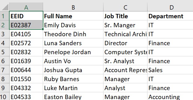
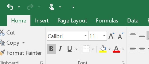
Find the ‘REMOVE DUPLICATES’ option and select it.

DATA Tab –> Data Tools Section –> Remove Duplicates

Step 3: Selection of Columns

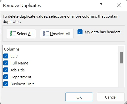
As soon as you click on remove duplicates, a dialogue box appears. You can check the boxes for the columns you want comparison and removal of duplicate data.

Furthermore, if your data comprises column headers, select the ‘my data has headers’ option and press OK. Once you check the header option, the first row will not be evaluated.

Step 4: Summary of Duplicates

The moment you click OK, the duplicates will be deleted. A dialog box shows the collective summary of deleted duplicates alongside the remaining count of unique values.

Filtering Unique Values and Removing Duplicates

You can also use filters to attain the objective to have unique values. However, many prefer to use only duplicates. Which eventually serves the same purpose. However, there is a slight yet critical difference. While you opt for the filtration, the duplicate values get hidden. Whereas if you delete duplicates, it gets rid of them instantly.

It is essential to understand the comparison briefly. Firstly, the value relies on what appears on the cell rather than the value contained. For instance, two cells have the exact date but in different formats. They are considered two unique values. Therefore, to get good results, check briefly and adjust cells manually.

Filter for Unique Values

Following is the process to filter unique values:

Start with selecting the table. Make sure all the contents have been selected.
Look for ‘Sort & Filter
Next, locate the advanced filter option from the group.

Data tab → Sort & Filter section → Advanced.

The advance filter popup will appear and as desired you can choose the following options to proceed further:

To filter the range of cells/tables in place, check the box with the option named ‘Filter the List In Place’.
If you wish to copy the results of the filter to a different location, then opt for the following:

a) Click the option named ‘Copy to another location’.

b) In the “Copy to” box, enter a cell reference where the resultant values must be copied.

c) You can temporarily click the “Collapse Dialog” option ( ) to hide the popup window. Then, once you have selected a cell on the worksheet, click the “Expand” option ().

d) Check the ‘Unique records only’ option box and then click OK.

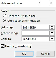
Opting for the Advanced Filter Option

With the help of the Advanced Filter option provided in MS Excel, you can now easily filter duplicate values, allowing the user to copy the unique values to a different place in a sheet. The following detailed steps will guide you on easily using the Advanced Filter option.
Firstly, click on the desired cell or range in the dataset you need to extract the duplicate. When you click on a single cell, Excel has the feature to automatically select the field when the Advanced Filter option is applied.

To locate the Advanced Filter option, follow
DATA tab → Sort & Filter section → Advanced and click on it.

Once you have clicked on the advanced filter option, you will see a list of options available. Only select the “copy to another location” option to copy all the unique values to a different location in a sheet.
To check the specified range, click on “list range”. Then enter the desired range in the “Copy to:” field. This will allow all the unique values to be copied in the new location.
Lastly, check the “Unique records only” box and click OK.

In this case, all the unique values will shift to cell G1.

The functionalities mentioned above are in-built features in Excel; now, let’s learn how to create our function to do the same.

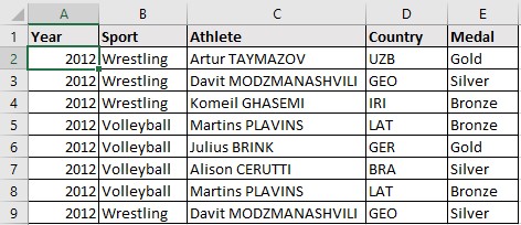
Using Formulas to Remove Duplicates

This approach can be achieved by following a simple example below.

In this method, you will involve the columns using Excel formulas to get the exact count. The next step would be to exclude the duplicate values.

1. First, combine columns A, B, and C such as =A2&B2&C2. This formula will be further copied down to all the rows.

1. The next step is to eliminate the duplicates by making a new D column named “Count”. Formula =COUNTIF($D$2:D2,D2)

Now, select a filter option in the Count column, this will automatically eliminate the duplicate values.

Power Query Tool to Remove Duplicates

With the help of Power Query in Excel, you will be able to import data in Excel from different sources. It will also help in removing duplicates and transforming your data properly.

First, select a cell in the dataset, then click on Query –> Edit.
Next, select the specific column by clicking on its column header. If you need to select multiple, press Shift+ Ctrl+ Click on the following column.
Lastly, select Home –> Remove Rows –> Remove Duplicates.