Home
/
Developer Tools
/
The Most Powerful Machine Learning Techniques in Data Mining

The Most Powerful Machine Learning Techniques in Data Mining

Advanced machine learning techniques are at the nexus of informatics in every industry and field of inquiry, and data mining is among the most intensive areas of focus in the broad field of machine learning today. Data mining techniques include algorithms such as classification, decision tree, neural networks, and regression to name a few. In this ByteScout article, we will explore data mining techniques in-depth, and cover the most important methods now at the core of enterprise research and development.

Classification and anomaly detection algorithms enable us to find patterns and actually discover knowledge in data that we could not see before. The relevance of these emerging fields to the growth and development of business and science is inestimable. Astonishing new realms of data exploration are opening up everywhere. Indeed, the onslaught of Big Data in conjunction with practical machine learning tools makes such discoveries possible. We will look at how regression algorithms work in practice and theory, using Python to illustrate our examples. Along the way, we will survey the list of rich methods of data mining in the context of Big Data providers like Quandl, AWS, Socrata, and UCI, all of which provide APIs for investigating the infinite new world of data mining and machine learning.

Data mining emphasizes the use of enormous data sets, and the popular programming model MapReduce evolved from the extraordinary requirements of utilizing Big Data through intensive regression models or neural networks which often contain thousands of machine learning features. Hadoop is an open-source implementation of MapReduce from Apache which facilitates the use of Big Data in data mining with clusters of processors. Clever data representation methods make possible the use of vast databases such as DNA sequencing data from the Human Genome Project to discover the structures of proteins and facilitate automation of new drug discovery. An advanced machine learning algorithm developed by Dr. J. Kermode can predict whether or not a molecule will bind to a protein target, thus predicting accurately candidate molecules for new drugs! Let’s look into the methods used in such innovation.

Our journey into innovation will translate best into the most popular language for using machine learning libraries: Python. Myriad Python libraries like SciKit-Learn contain both ML functions and datasets ready for training and testing. Machine learning code involves complex math, and we need not complicated matters by starting out in a language with complicated syntax; Python is easiest to read, debug, and run. Python also supports many data structures which make managing large data sets easier. And Python is especially easy to use for data typing. Ideally, to follow this presentation go ahead and install Python on your system.

The easiest way to install Python is to let the Anaconda distribution configure all the libraries and dependencies, as well as setting the system path. Anaconda includes all the libraries we will use here such as Scikit-Learn, Pandas, and the core math libraries like Numpy. Another great library to facilitate the development of algorithms in Python is the Jupyter Notebook, a freeware framework that enables coding, running, and annotating Python in your browser. The cleanest way to use Python is right on the command line or terminal. You can start Python and prototype lines of code there, and then paste them to your favorite editor or IDE. This way of working leads to familiarity with the interaction of Python components in your system.

Anaconda is a rather large installation file, and if you prefer a leaner download simply get a copy of Python from the organization and then pip install only the libraries required in this presentation. For example, after updating your system path to include Python, you can run python -m pip install jupyter on the command line or terminal and Jupyter will auto-install. Then you can also run it from the command line with the command jupyter notebook. As you will discover, Jupyter notebooks (previously called “iPython”) are a very convenient way of developing machine learning code and commenting inline to facilitate your study.

Embracing the Math

Inevitably, machine learning in data mining is a mathematical endeavor. Matrix operations are the core of neural network design. This is true for two reasons. “Neural networks” are represented by systems of equations, and the parameters or coefficients of these equations constitute the elements of a matrix. These parameters are the “neurons” referred to in the analogy to the brain. Secondly, therefore, most data structures used in machine learning and data mining are modeled as matrices, vectors, or tensors, most commonly referred to as arrays. The numerically indexed array gives us computational access to the elements of arrays to facilitate calculation.

We will have to face the math if we are going to truly comprehend the fundamental concepts of machine learning. Although Python and libraries like TensorFlow make it possible to do machine learning without understanding how it works, we will probe deeper. From reading and wrangling a dataset all the way to multivariate linear regression, there are libraries that do the math for you. You can easily follow a tutorial and run a data classification algorithm, but this will not lead to insight. We are going to penetrate deeper and look at the core of the reactor!

We are actually going to apply machine learning and build a predictive model to determine the chances that a patient will become diabetic based on data about body mass and other data features. Many introductions to data mining waste time on generalizations; we’re going to build an actual predictive model right now. First, we are going to take one giant step forward and read a diabetes dataset into a Python array! This will cultivate a real knowledge of the math mechanics of data mining and machine learning.

As a preliminary step, open a new Jupyter Notebook. Create a folder for your new project and open a command line. At the prompt, type jupyter notebook, and Jupyter will open in a new tab in your default browser (of course, you can follow this example in your favorite editor without Jupyter). Glance back at your command line and you will see Jupyter generating a lot of automatic dialog there, some of which can be useful diagnostically. Let’s go ahead and import the libraries we will need for our example:

import numpy as np
import pandas as pd
import matplotlib
from sklearn import datasets , linear_model

Here we import Numpy, a Python library that instantly gives us great power over data structures similar to that of Octave and MATLAB. This is what we will use to handle linear algebra and matrix operations. Pandas is a library designed for DataFrame analysis and supports many operations similar in functionality to the spreadsheets of MS Excel, such as pivot tables. Matplotlib is widely used for the 2D plotting of data and functions. And SKLearn is the popular Python library for machine learning functions which also contains many datasets for training and testing models.

The next step is to read our dataset into an array. In this example, we will use a diabetes dataset from a research study publicly available to predict the progression of disease in patients. This is the type of dataset commonly curated on Big Data sites like Quandl and UCI. This particular dataset will serve several purposes for our demonstration. In your Jupyter notebook or editor, enter the following code to read in the diabetes dataset:

ds = datasets.load_diabetes()
X = ds.data
y = ds.target
np.shape(X)

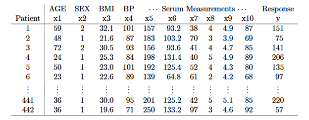
Remember that this dataset is included in the SKLearn library, but millions of datasets are available and the providers often make their own APIs freely available as well. Python figures out for us the variable type for ds and loads the arrays X and y with the dataset as we will see. Next, Numpy’s np.shape function will return the size of the X array as (442, 10) meaning n=442 samples of 10 features. If we print the first row X[0] we can see an excerpt from the dataset. This brings us to a discussion about data wrangling.

Munging & Wrangling

In the original publication of this dataset, the authors naturally included column labels as we can see in the table above. The purpose of that 2003 research was likewise to build a predictive model based on methods of the period. However, this dataset now curated by a variety of providers does not contain labels for the features chosen for use in the model. This raises the discussion of a practical and often difficult procedure in data mining known as wrangling or munging.

There is actually a recent GitHub debate about this particular dataset in which one developer puzzles over the usefulness of a dataset without feature labels. Fortunately for our demo, the original publication is still available and we are thus able to reassign the labels manually as shown in Table 1 to make the features meaningful. And this is a common weirdness encountered along the way to building a model. Interestingly, this calls attention to the fact that a linear regression model of this data can accurately model and predict outcomes without knowing what any of the data means. Alas, we humans still need the feature labels to interpret the outcome!

Linear Regression – A First Model

The next step in our journey is to build a model to predict disease progression in a sample of patients. The features available for our model as shown in Table 1 include age, sex, body mass, blood pressure, and six blood serum samples. The plan is to fit a regression model to predict the target value in the dataset, shown as “Response y” in the table. For data visualization, we will use the body mass feature (BMI).

Go ahead and enter the following code to reduce the X array to column 2 (this is a zero index array). We use matrix operators here to divide the dataset into 362 training samples and 80 more for the test:

X = X[:,2]
X = X.reshape(-1, 1)
y = y.reshape(-1, 1)
X_train = X[: -80]
y_train = y[: -80]
X_test = X[-80:]
y_test = y[-80:]

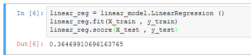
Now the dataset is ready to run a regression. We use SKLearn functions to train the model in the following code:

linear_reg = linear_model.LinearRegression ()
linear_reg.fit(X_train , y_train)

If you are building this model in Jupyter you should see this:

And check the score against the test data like this:

linear_reg.score(X_test , y_test)

If you are following along in your editor you should get a result about .365 for the test score. This is a raw prediction based on a single feature, the patient body mass. With increasing feature complexity we can achieve better accuracy. SciKit-Learn also provides the Support Vector Regression for the nonlinear or polynomial fitting of data.

Applied Machine Learning Techniques

Beneath the surface of SKLearn a regression model is optimized by adjusting the parameters to fit the training data to the target outcome. In other words, there is a cost function that is minimized by a method such as a gradient descent to fit the training data to the known outcomes most accurately. In the field of data mining, there are many popular variations and approaches such as logistic regression. How does this work exactly?

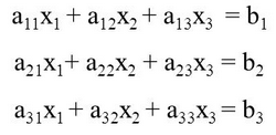
In regression, we take a set of linear equations that we build from the features in our dataset and solve it for a set of parameters that we optimize with a cost function. In our diabetes example, we have 442 samples patients and each sample has 10 features including sex, age, body mass, and blood test results. To set this up as a set of linear equations we write it in a form like this:

Wherein each row models the data for a patient. Now here is the trick: we already know the values for X. They are the data features in the training set. Each time we run a training session we put the data into the X values and optimize the parameters or coefficients. What we want to optimize are the values for the coefficients, the a₁₁, a₁₂ … a_n. In our case, the subscripts go up to 10 because we have 10 features in the data. 442 rows going down by 10 features going across. So the last parameter in our set of equations looks like a_{442 10}in the figure above.

The “target” values are the known values in the training and test data. They tell us about the actual disease progression in this example. Again, the a values are what we want to “solve” for or optimize using a technique of machine learning called regression. To point out a few more items of popular jargon thrown about loosely in articles about machine learning, the “layers” of a “neural network” are the number of parameters across from left to right in the above equations. The a values are the “neurons” which are “activated” when the model is “trained.” So as you can see the often-used analogy to the human brain is a very loosely fitting analogy indeed.

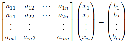
The next step in setting up a machine learning model is to simply rewrite this set of equations as a matrix or set of matrices. We can do this by writing the a values in their own matrix like this:

Now here we have something that Python and especially Numpy know how to process very efficiently! Here also you can see why a complete set of data is crucial to the solution. If one of the a values is missing then we get into yet another technique of data mining which has the goal of estimating missing data.

The solution to the above equations is a process of setting up a cost function and minimizing the cost by adjusting the a values until the b values most closely match the target values in our training set. The SKLearn library does this calculation for us. Once the training data are used to find the optimum parameters we then test the model by using the test values to score the accuracy of the model.

Crossing the Finish Line

Although this is a linear setup there is a similar method for handling nonlinear data modeling. Developers usually output a graph showing a scatter plot of points with a line down the middle of the data showing how the model approximates the target data. Like the “neural network” analogy to the human brain, this data visualization is only an analogy and it may actually mislead. A simplistic visualization of our example can be generated with this code:

plt.scatter(X_test , y_test)
plt.plot(X_test , linear_reg.predict(X_test))
plt.show ()

The result, when we do a trillion iterations over a million parameters, does not fit neatly on a MATPLOTLIB chart. This is why we get surprising and sometimes mysterious results, some insightful ideas, and others which suggest we think more carefully about feature selection and how that impacts the results. This nonlinear often unpredictable aspect of a model intended to predict is what contains a hint of quirky intelligence. In the final analysis, there are myriad formulations of machine learning to explore. Stay tuned to ByteScout for the next installment on the exciting field of machine learning.