Our ByteScout SDK products are sunsetting as we focus on expanding new solutions.
Learn More
Important Update
ByteScout SDK Sunsetting Notice
Our ByteScout SDK products are sunsetting as we focus on our new & improved solutions.Thank you for being part of our journey, and we look forward to supporting you in this next chapter!
The users use Excel to organize and calculate their data. Therefore, the dropdown lists in Excel benefit them if they want to select an item from multiple item lists instead of typing them repeatedly.
Following are the steps to create a dropdown list in Excel:
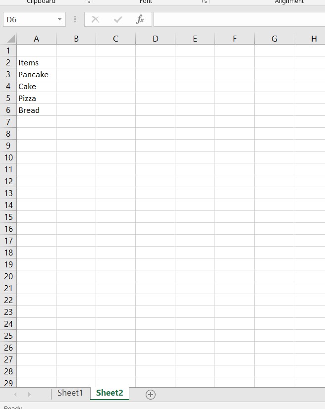
1. Tap the add “+” sign at the bottom to create a new sheet and write the list entries in a table. The users can hide or protect the sheet containing the list to stop others from modifying or seeing the list.
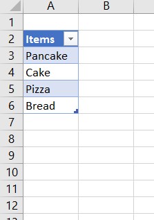
Note: The users can convert the list to a table by selecting any cell in the list and pressing the “ctrl+T” keys. For instance, in our case, cell A2 is the header cell, and the cells below are the table entries containing the name of the items.
2. In sheet 1, select the cell where the user wants the dropdown list to appear.
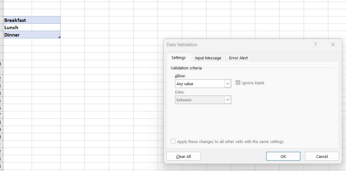
3. Click the data validation option in the data section of the ribbon, and a pop-up will appear.
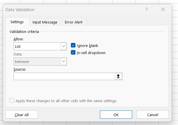
4. Select the “List” from the options in the “allow” box.
Note: The users can check or uncheck the “ignore blank” and “In-cell dropdown” options based on their use cases.
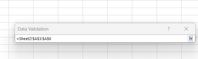
5. Write the columns in the source box if the list is in the same sheet, or the users can click on the arrow in the box. Then click sheet 2 (or the sheet containing the list) and select the columns. The box will have the values written such as below:
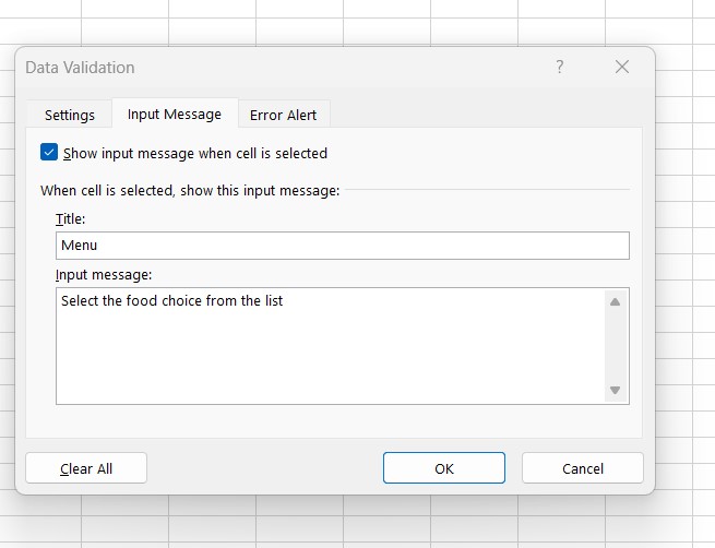
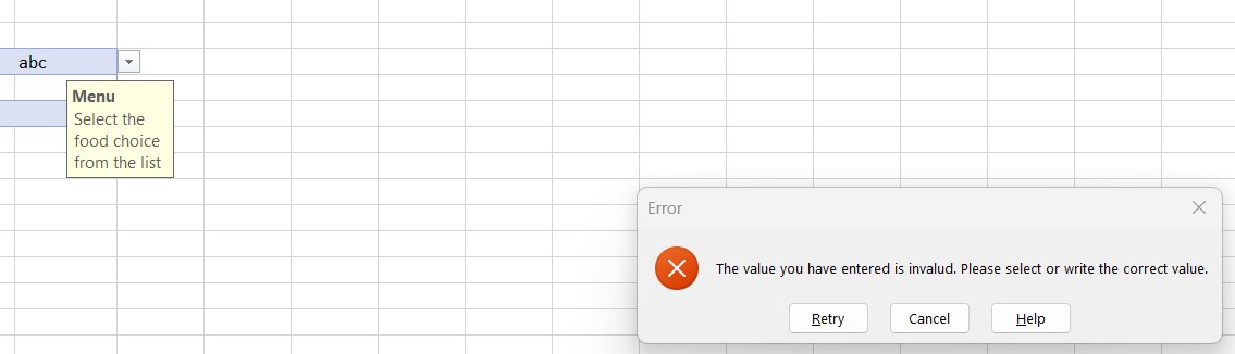
6. Write the input message in the “Input Message” section if the user wants to display the message whenever he clicks the list or the cell.
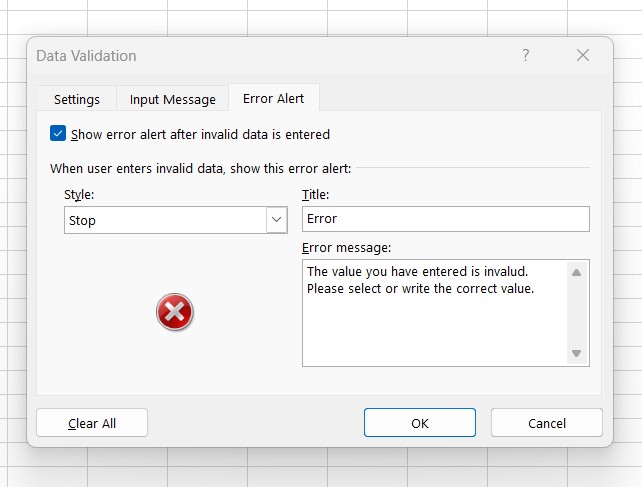
7. In the “Error” section, write the title and error message for when the user enters the incorrect data, i.e., the item which is not in the drop-down list. So, the error message will pop up to inform them that the data is invalid.
Note: The users can also change the alert box type by selecting other styles in the style box. There are three options: stop, warning and information styles, which the users can select depending on the nature of the message. By default, the value is set to “stop” style to display “error”. If the user wants to display a warning, he can select the warning style, and a yellow exclamation mark inside the triangle would represent the warning pop-up.
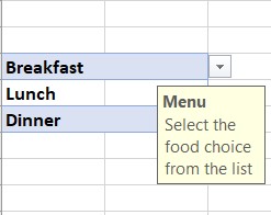
8. Click the “OK” button, and the dropdown list will appear in the selected cell.
Click on the arrow button to see the list and select the item from it to display in the cell.
Adding the invalid data will result in the appearance of this dialog box:
Steps to Edit the DropDown List
In various scenarios, the users would need to edit their dropdown lists by adding or removing items from them and want them to get updated in their dropdowns. While editing the already written data, for instance, changing the “cake” to “cakes” or writing something else in that cell would update the dropdown list automatically. However, if the users want to remove or add items to the list, they must follow the steps below. There are multiple ways to edit the drop-down list in Excel.
Editing using Data Validation
Open sheet two and edit the items list by adding, removing or changing the already written items.
Return to sheet one and choose the data validation option in the data section of the ribbon.
Change the “Source” Range and press “Ok”. It will update the dropdown list to the new list.
Editing the Table Entries Directly
The users can also edit the dropdown list directly from the items table without updating the source range in the data validation. Below are the steps to add new items to the list:
1. Open sheet two and select any table entry.
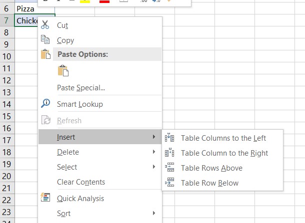
2. Right-click on the cell and select the insert option to add an item.
3. Select the “Table row above” or “Table row below” and add the new item in the new row.
4. The table will automatically update the source range in the data validation box and update the dropdown list automatically.
Similarly, the users can delete the items by following these steps:
1. Open sheet two and select any table entry the user wants to delete.
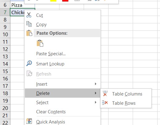
2. Right-click on the cell and select the delete option.
3. Select the “Table rows”, and that will delete that row from the table.
4. The table will automatically update the source range in the data validation box and update the dropdown list automatically.
Congratulations! You have successfully learned how to create drop-down lists in Excel. By mastering this essential feature, you can now enhance your data entry efficiency, ensure consistency, and improve overall productivity. Whether you’re managing large datasets, creating forms, or conducting surveys, drop-down lists provide a powerful tool for organizing and analyzing information. Remember to explore advanced options like dynamic lists and conditional formatting to take your Excel skills to the next level.
About the Author
ByteScout Team of WritersByteScout has a team of professional writers proficient in different technical topics. We select the best writers to cover interesting and trending topics for our readers. We love developers and we hope our articles help you learn about programming and programmers.
Software developers are sorcerers. Coding is an artistic and goal-oriented venture. Most importantly, there are some crucial problems that only software programmers can solve by...