Types of scales. Multi-criteria selection tasks. The Analytic Hierarchy Process (AHP) for complex decisions.

Analytic Hierarchy Process (AHP) was initially developed by Thomas L. Saaty in the 1970s and is used as a method to organize and analyze complex information for the purpose of decision making based on multiple parameters.

Types of scales

Nominal – no information on the preference of objects carries, except for equivalence of objects, an example of a scale is gender, marital status.

Ordinal – used to arrange objects in the order of their preference, but the values ​​themselves do not carry information about the “degree” of preference. Arithmetic operations are usually not performed. An example of an ordinal scale is school grades.

Interval scales – order objects and the relative distance between objects is also considered important. An example of an interval scale is the temperature scale.

Ratio scales – This scale differs from the interval scale only in that it strictly defines the position of the zero points. Due to this, the scale of relations does not impose any restrictions on the mathematical operations used to process the results of observations. An example of a ratio scale is the length of an object.

The absolute scale is the origin and units of measurement. An example of a scale is the number of defects in a product.

Interval, ratio scales, and absolute scales are quantitative scales. Nominal and ordinal scales refer to quality scales.

Operations on the values ​​measured in different types of scales without bringing them to a single type of scale are impossible.

Multiple choice selection tasks

There are such optimization problems where it is necessary to make the optimal choice according to several criteria. Such tasks can be solved in various ways. One of these solutions is the choice of the main indicator from their set and the rest of the rest from the top or bottom, depending on their meaning.

Sometimes, not for all indicators, it is possible to assign clear boundaries and then select many promising solutions that are not improved by any indicator without deterioration of at least one of the others.

These solutions are called effective and a choice is made among them. Mathematical methods for constructing sets of effective solutions are called multicriteria optimization.

The Analytic Hierarchy Process (AHP)

The Analytic Hierarchy Process (AHP) is a mathematical tool for a systematic approach to complex decision making. Analysis of the decision-making in the AHP begins with the construction of a hierarchical structure that includes the goal, criteria, alternatives, and other factors considered that influence the choice. This structure reflects the understanding of the problem by the decision-maker.

The process of choosing an alternative based on the AHP consist of:

1. Construction of a qualitative model of the problem in the form of a hierarchy, including the goal, alternative options for achieving the goal and criteria for assessing the quality of alternatives.
2. Prioritization of all elements of the hierarchy using the method of pairwise comparisons.
3. Synthesis of global priorities of alternatives by linear convolution of the priorities of the elements on the hierarchy.
4. Verification of judgments on consistency.
5. Decision making based on the results obtained.

Example

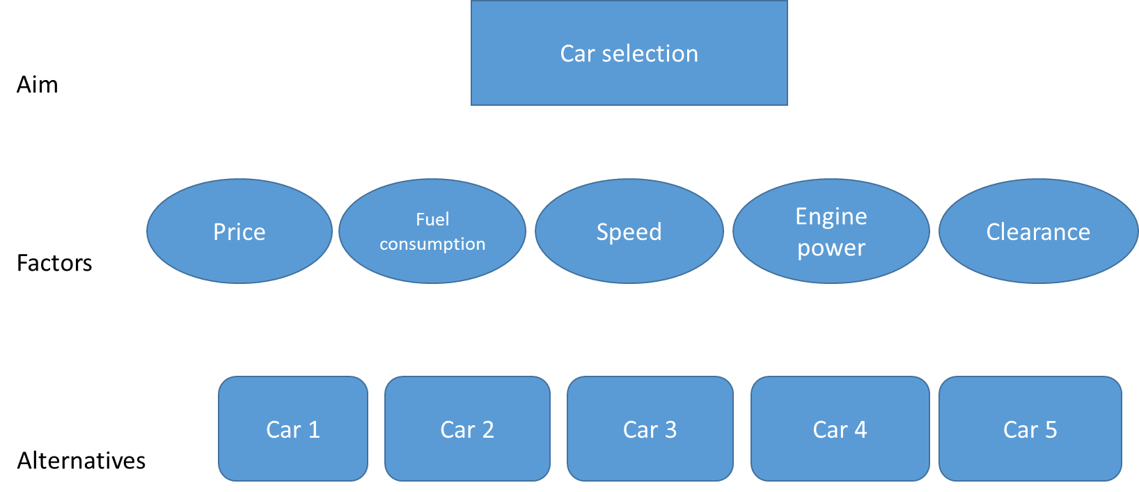
As an example, we can consider how a car is chosen by analyzing hierarchies. The following cars will be used as selected cars: Car 1, Car 2, Car 3, Car 4, Car 5.

Factors: price, fuel consumption, speed, engine power, ground clearance.

Table 1 Cars and factors

The evaluation criteria are the maximum value of the alternative when calculating the global priority.

Building a hierarchy (in the form of a decision tree):

For each of the factors, it is necessary to identify the scale used for its measurements and compare the factors, dividing them into groups according to the type of scale. In this example, all factors refer to quantitative factors.

Building a relationship scale:

It is necessary to compare each of the criteria with each other in order of importance. Table 1 presents the scale of relationships.

Table 2 Scale of relationships

The results of the comparison can be seen in table 3.

Table 3 Pairwise comparison of factors

We calculate the geometric mean and weight, normalizing by the geometric mean, obtain the normalized value of the “importance” of the criterion. The geometric mean is calculated as , where  is an element of the collection.

Table 4 Pairwise comparison of factors with the weight of each

We get the following:

Price> Fuel consumption> Speed> Power> Ground Clearance

Where the sign “>” determines the preference of factors.

Next, you should compare the alternatives (cars) by the selected criteria:

Example of comparison of cars by the factor “Price”.

Table 5 Comparing alternatives by price criteria

Priority criteria Price:

Car 5> Car 1> Car 4> Car 2> Car 3

And so it goes on for each of the criteria.

To make a final decision on choosing a car based on the AHP, it is necessary to transfer the values of the priority vectors for each factor (criterion) to the final table and calculate the final global priority.

The final global priority is determined by summing the global priority vectors by vehicle selection criteria.

Summary table and result:

Example of calculating the final priority for Car 1:

0.43 * 0.26 + 0.27 * 0.26 + 0.14 * 0.35 + 0.08 * 0.38 + 0.03 * 0.20 = 0.28

A high rating will correspond to the highest value of the global priority vector. The winner is Car1.

Conclusion

One of the methods of multi-criteria evaluation is the AHP method which is used for different values, measured in different scales. This method helps to structure various factors even if they are measured in different scales and helps to make a decision based on multiple factors. In the example, we’ve applied this method to the selection of cars.

   

About the Author

ByteScout Team of Writers ByteScout has a team of professional writers proficient in different technical topics. We select the best writers to cover interesting and trending topics for our readers. We love developers and we hope our articles help you learn about programming and programmers.